Example

The full procedure is shown here using a complete example.

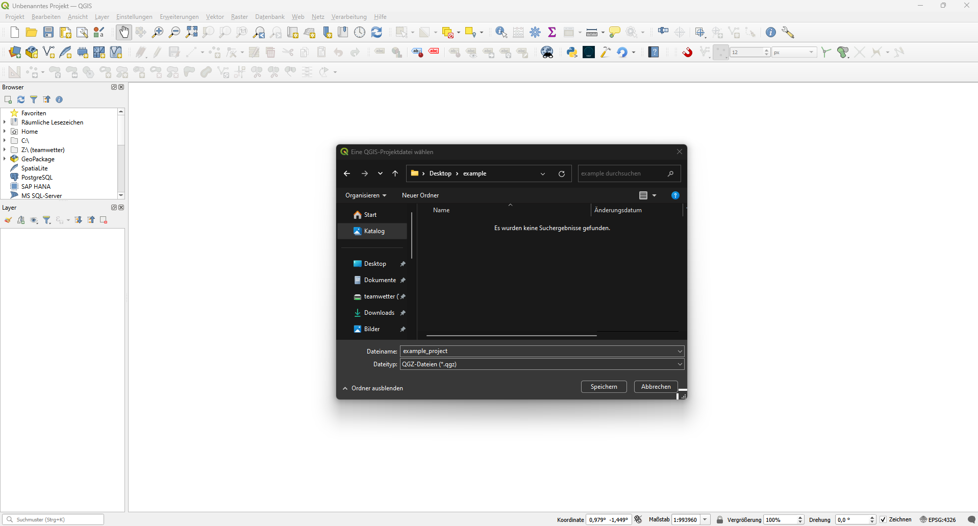
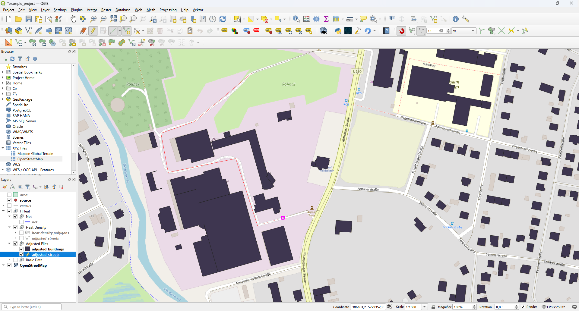
1. Create a folder for your project. Save your empty QGIS project in that folder

   

2. Start F|Heat. The user interface will open with the introduction tab. Simultaneously, the layer groups for the individual steps of the planning process will be created automatically.

   

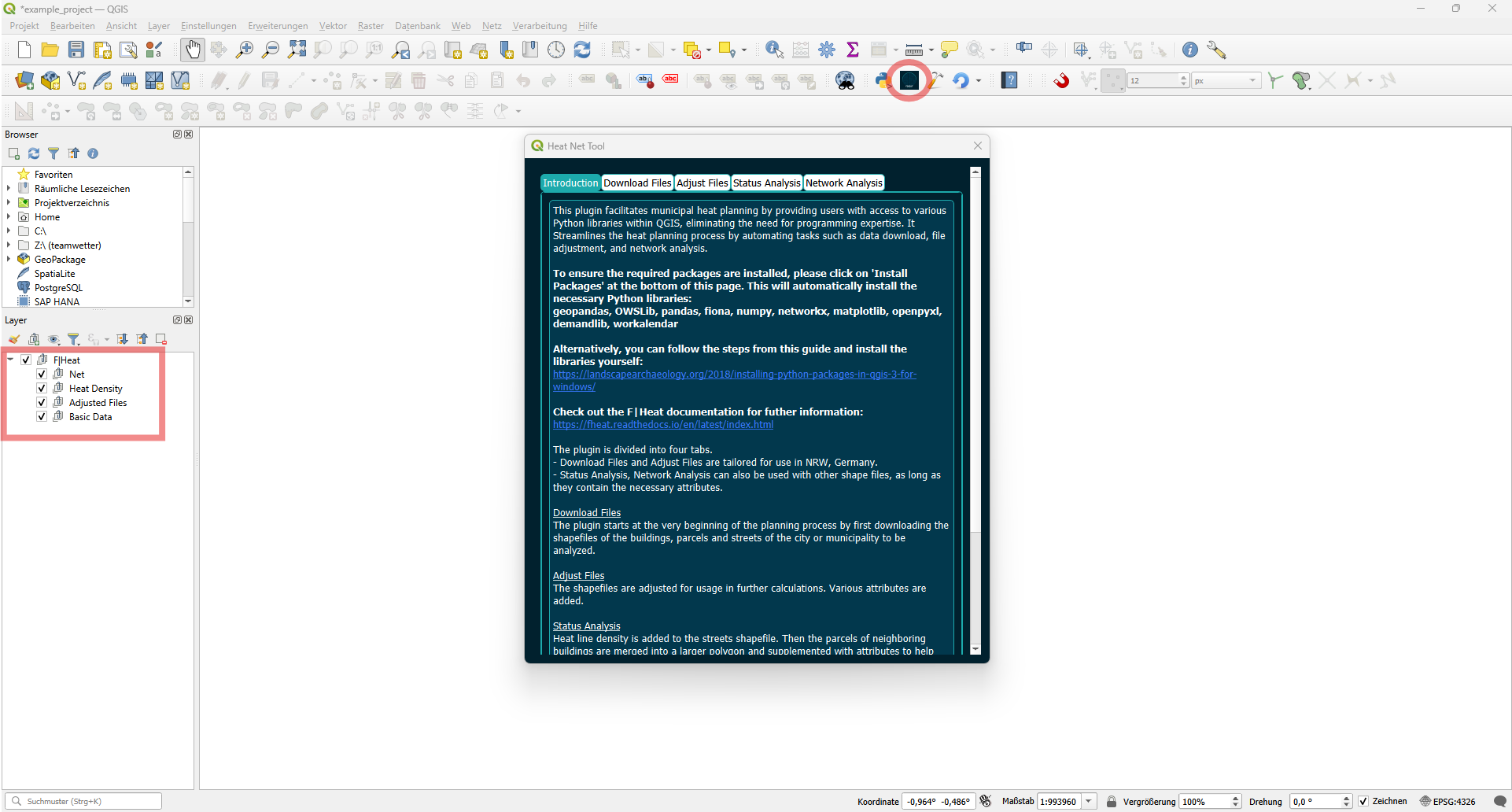
   (If you have not installed the required python packages yet, check out the Install python packages section.)

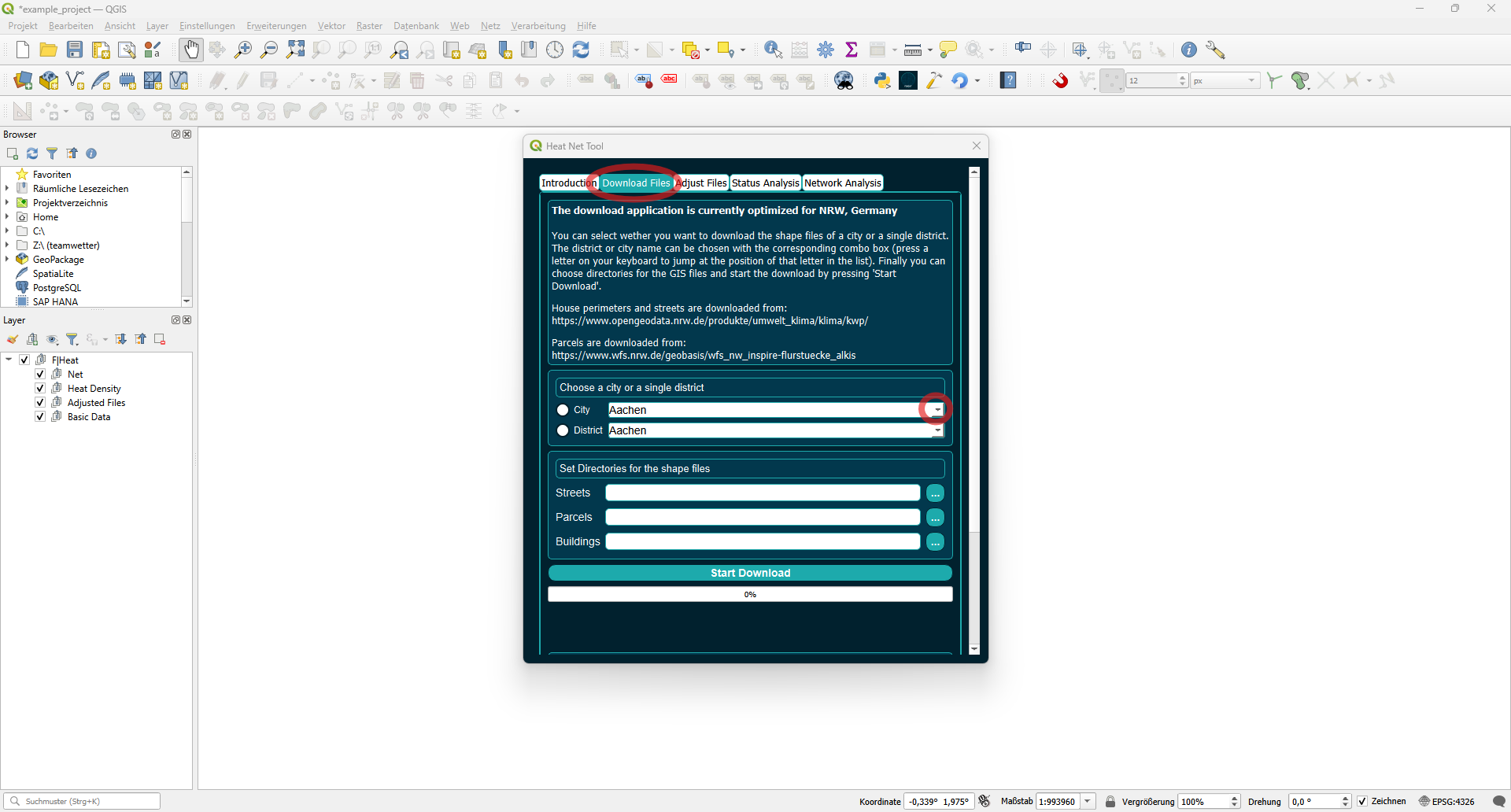
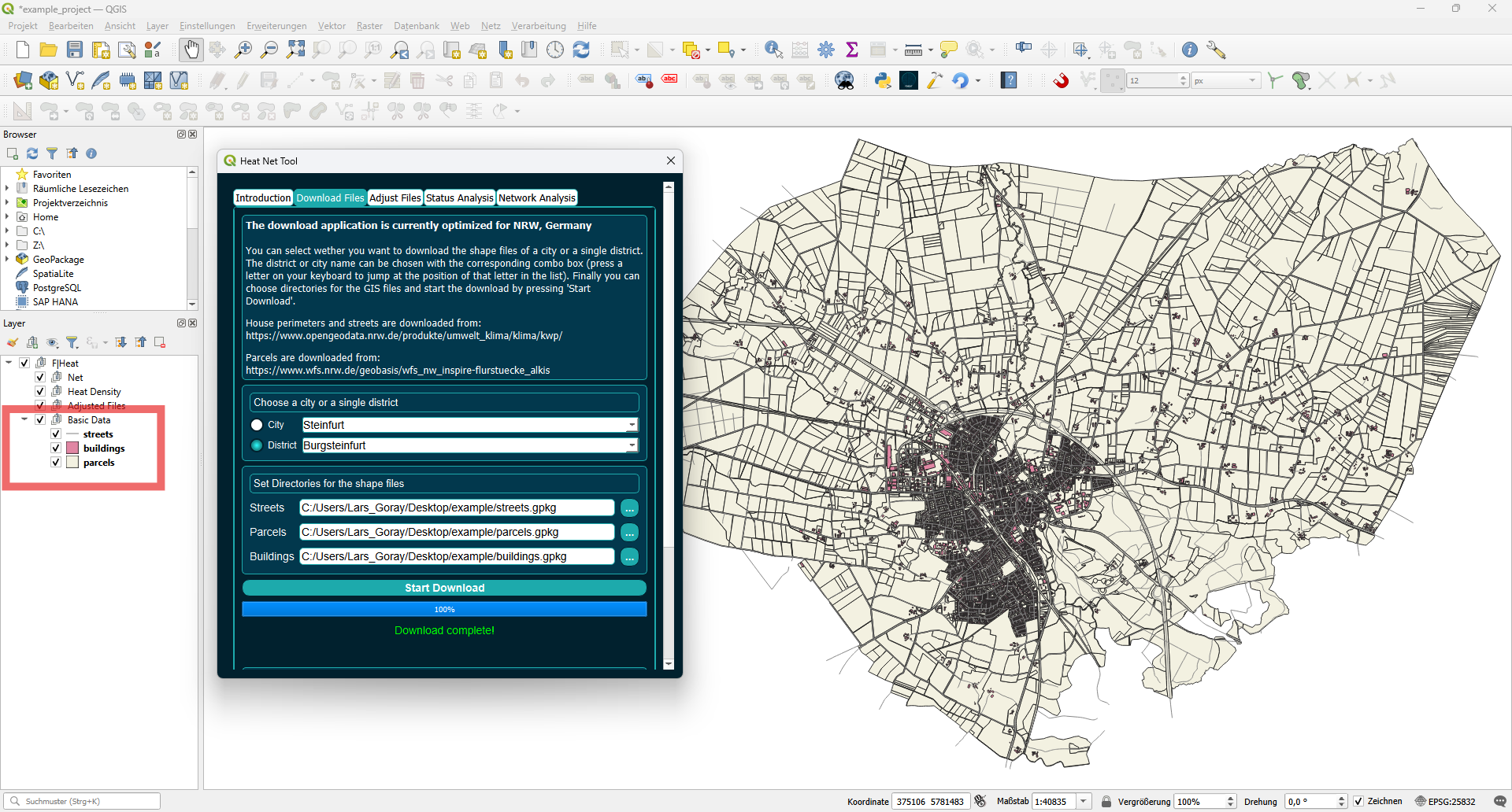
3. Switch to the Download Files tab. Here you can download the basic shapefiles needed for the planning process. Select a city from the dropdown list.

   

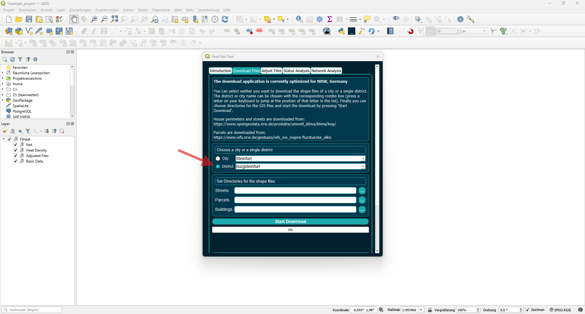
4. You can select whether you want to download the shapefiles for an entire city or a single district by toggling the buttons on the left. Once a city is selected, you can choose a district of that city by clicking the second dropdown list. In this example, we select the district Burgsteinfurt of the city Steinfurt. You can choose a different city and still follow along with this example.

   

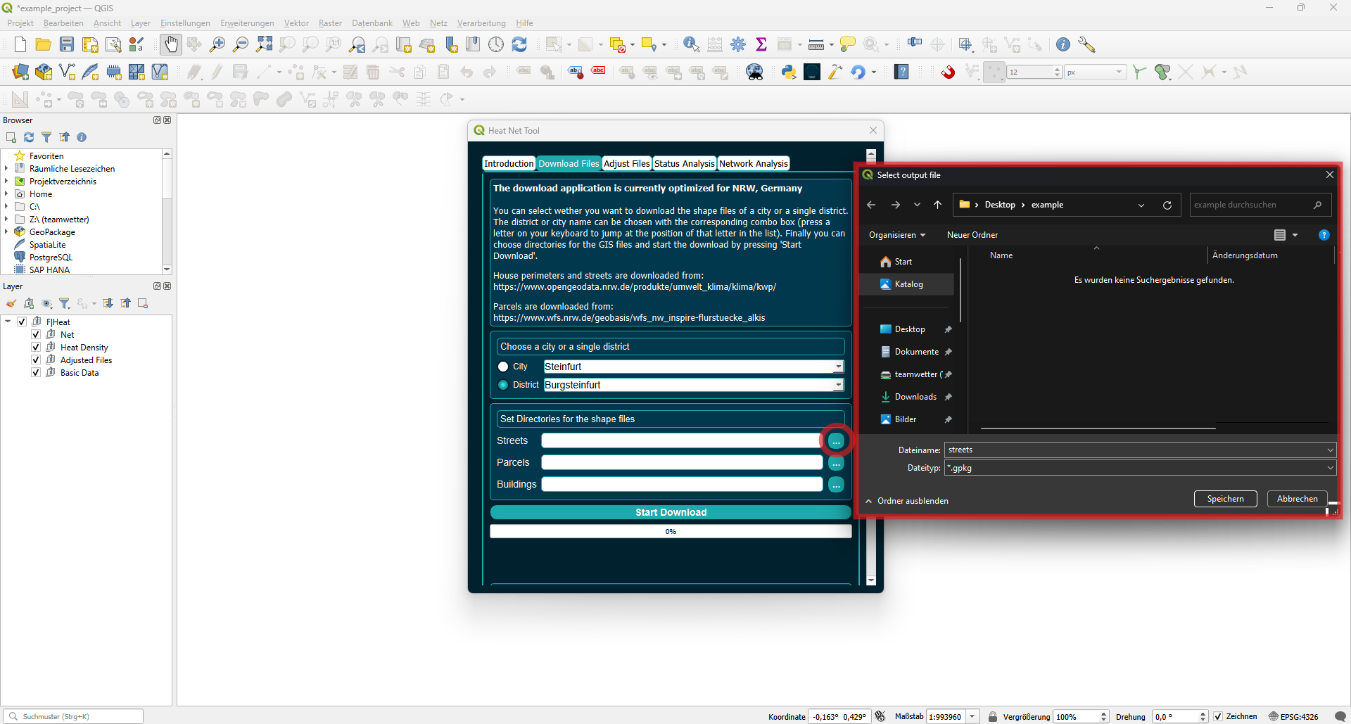
5. Next you need to set the file path for the shapefiles by clicking the (…) button. This will open the directory of your QGIS project, where you can enter a file name.

   

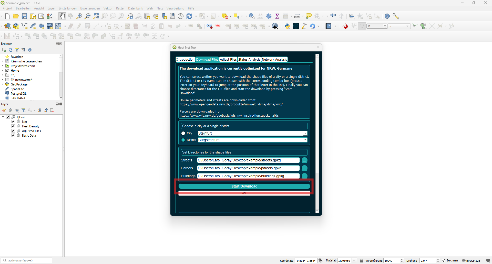
6. When all file paths are set and a city or district is chosen, you can start the download by pressing Start Download. The progress bar below will show the progress of the process.

   

7. All layers are loaded into the Basic Data group once the download is complete.

   

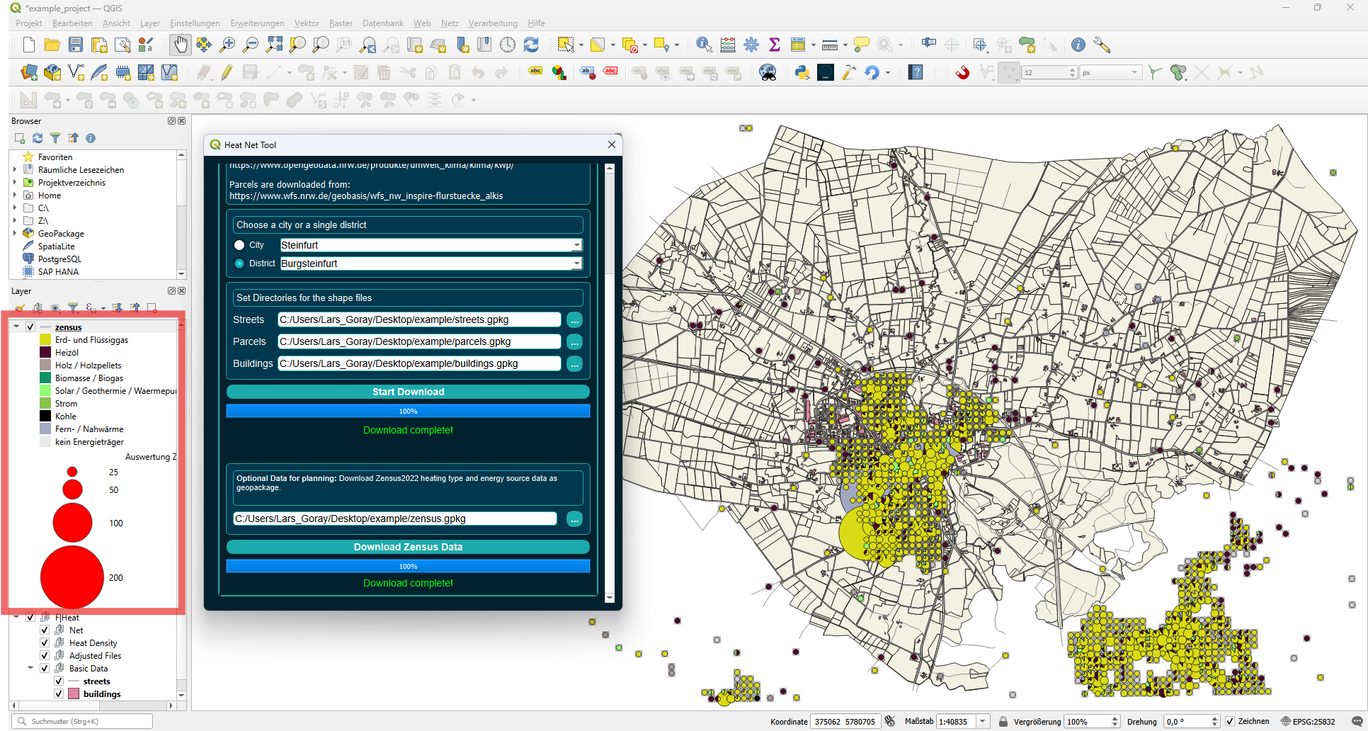
8. You can also download optional Zensus2022 data that provides information about the type of heating and energy sources of the buildings in your city or district. This may be helpful in the planning process, but it is not necessary. Scroll down or extend the window to access the zensus data download.

   

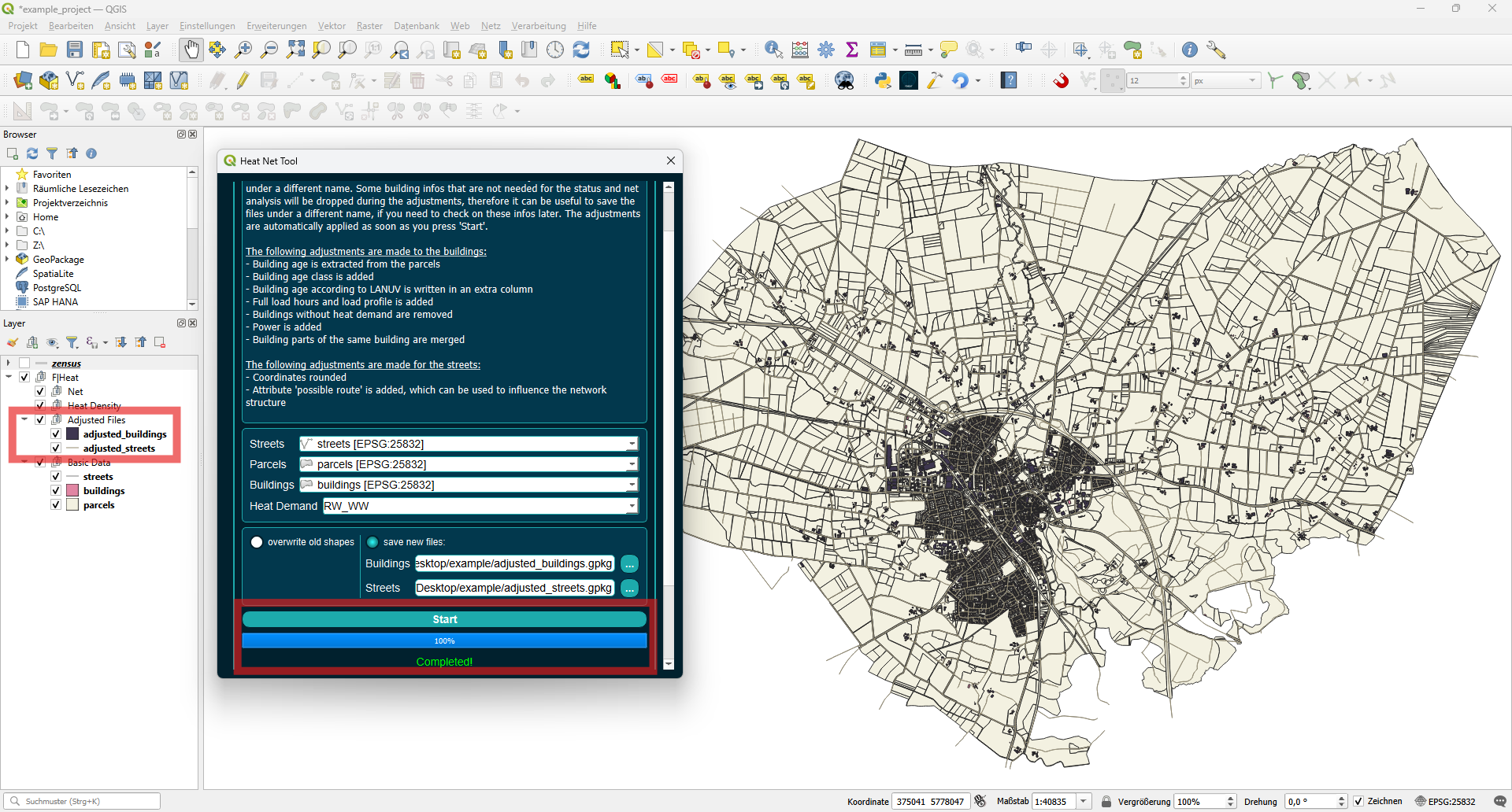
9. For further calculations, the downloaded shapefiles of the buildings and streets must be adjusted. Toggle the dropdown lists to select the correct layers for streets, parcels and buildings. Choose the desired attribute of the buildings layer as heat demand. For the downloaded data, you can choose RW_WW where RW = Raumwärme(space heating) and WW = Warmwasser(water heating) are combined.

   

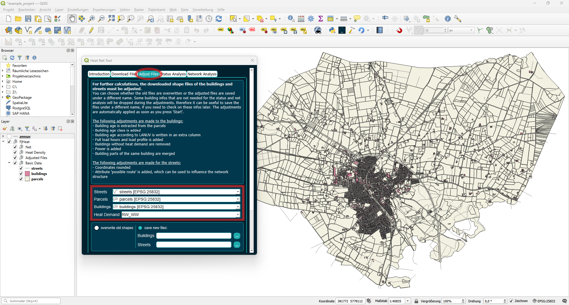
10. You can choose whether to overwrite the old files or save the adjusted files under a different name. Some building information that is not needed for the status and network analysis will be dropped during the adjustments; therefore, it can be useful to save the files under a different name if you need to check this information later.

    

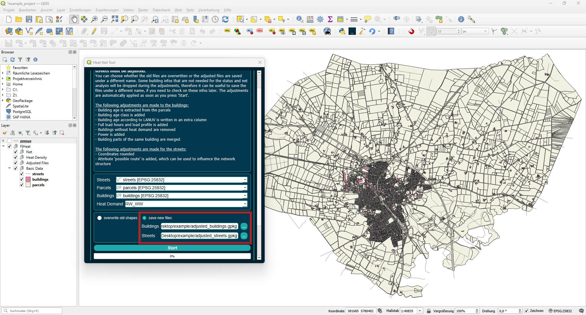
11. The new files will be added to the Adjusted Files layer group once the process is complete.

    

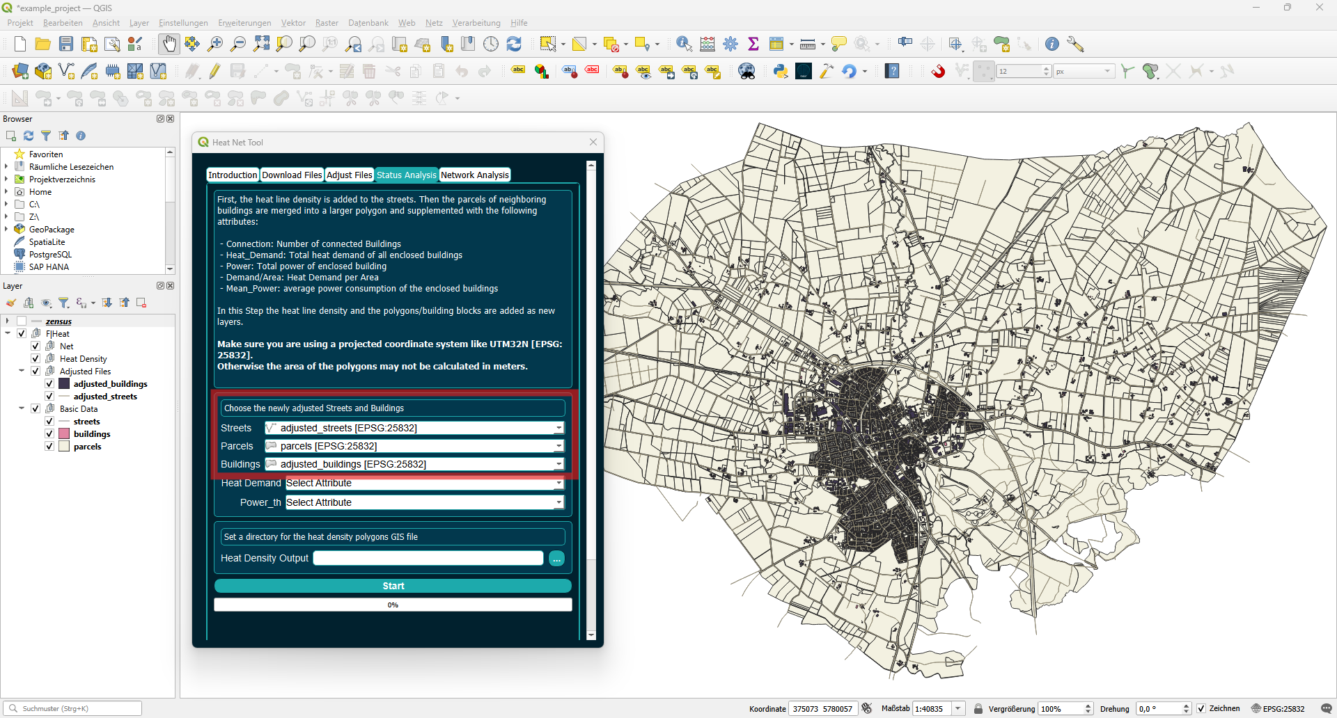
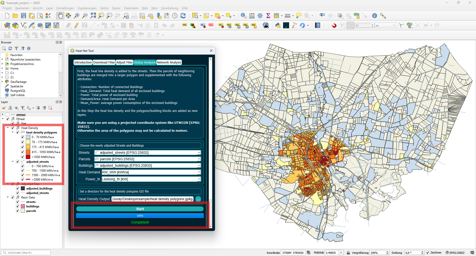
12. In the Status Analysis tab, the heat line density and the heating demand per building block are added. Make sure you are using a projected coordinate system, such as UTM32N [EPSG:25832]. Otherwise, the area of the polygons may not be calculated in meters. Choose the newly adjusted streets and buildings.

    

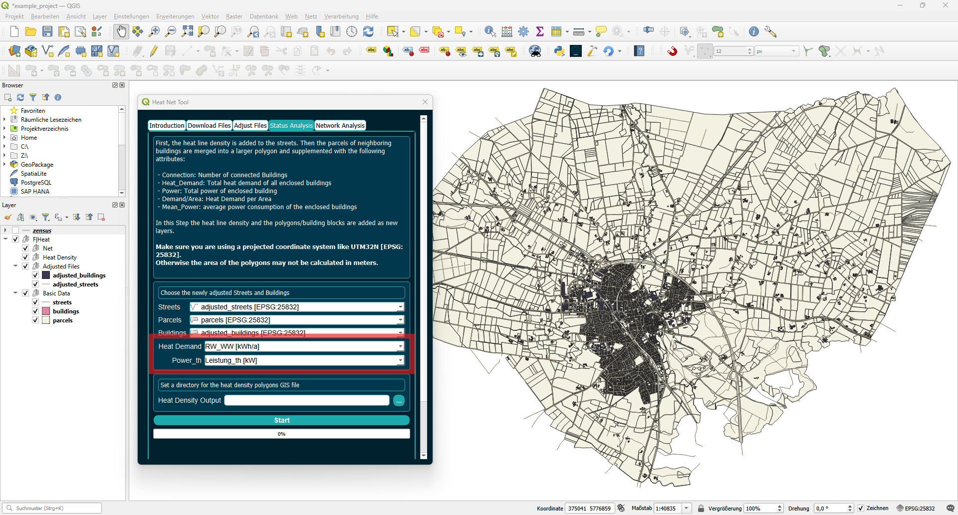
13. Select the desired attribute of the buildings layer as heat demand. For the downloaded data, you can choose RW_WW where RW = Raumwärme(space heating) and WW = Warmwasser(water heating) are combined. The attribute for thermal power is Leistung_th.

    

14. Set the file path for the heat density building blocks. The heat line density attribute will be added to the adjusted streets.

    

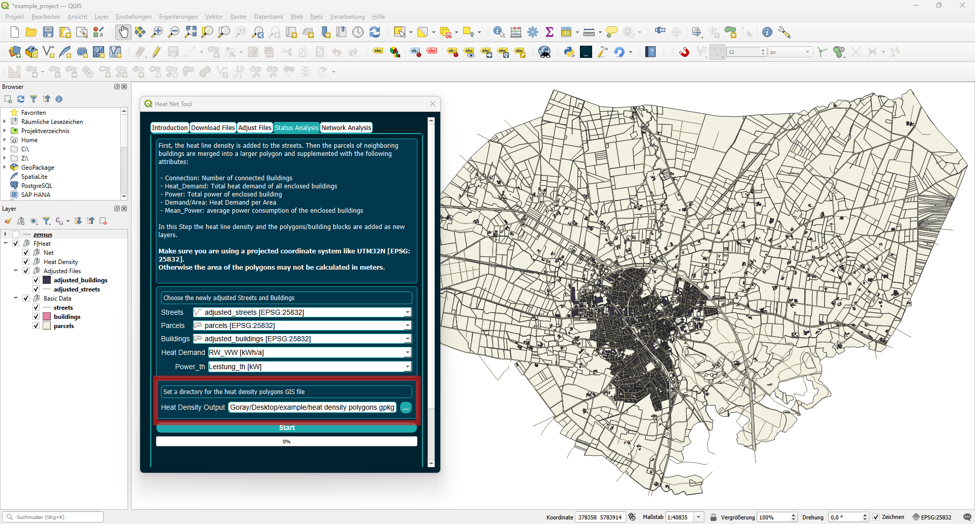
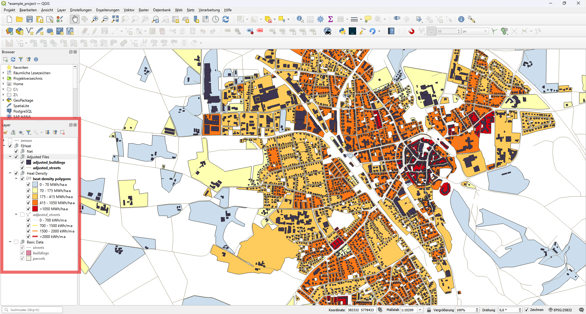
15. Press start and wait for the process to complete. The layers will be added to the Heat Density group.

    

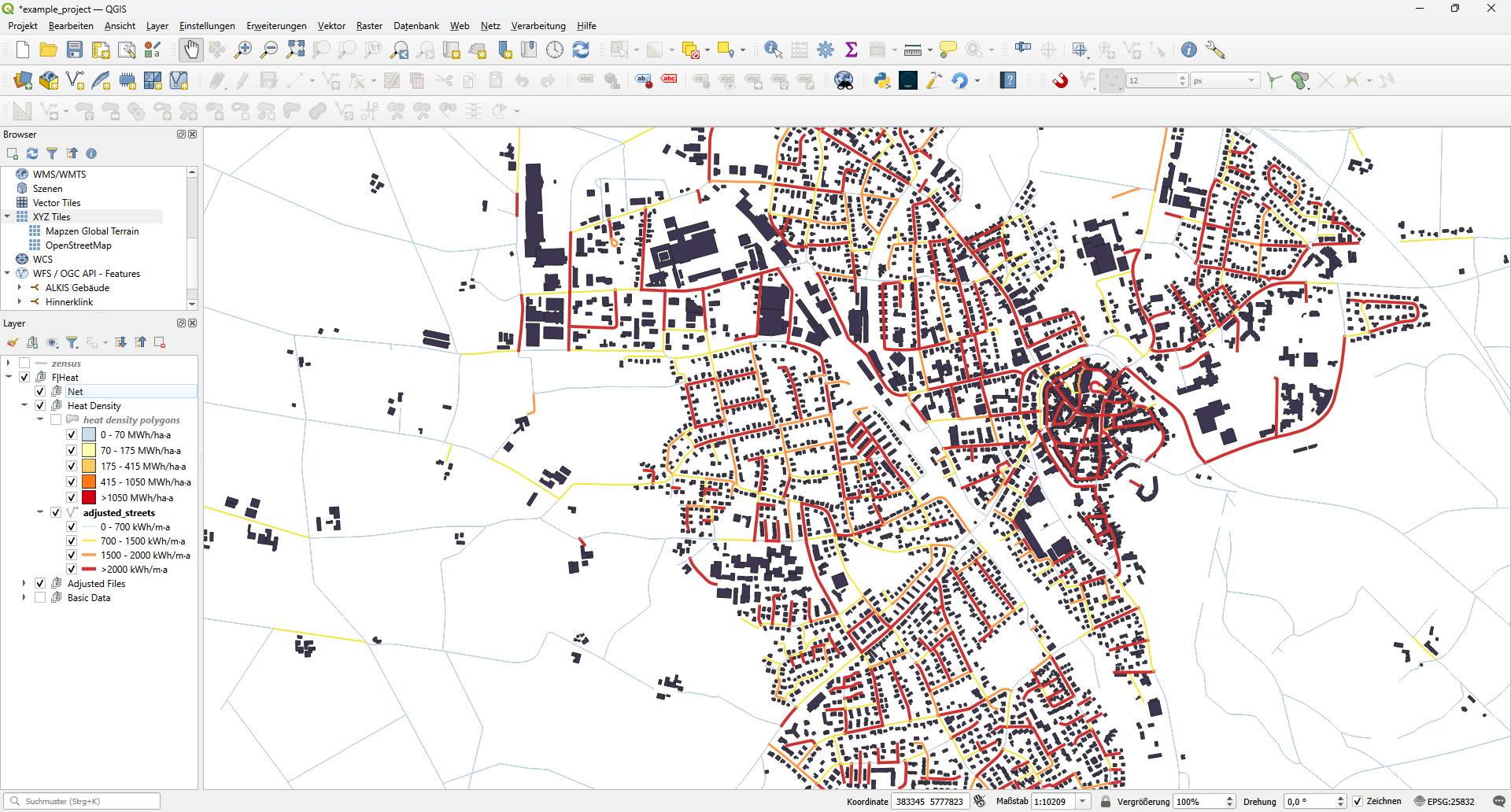
16. You can change the layer order and visibility by dragging the layers and toggling the checkboxes.

    

    

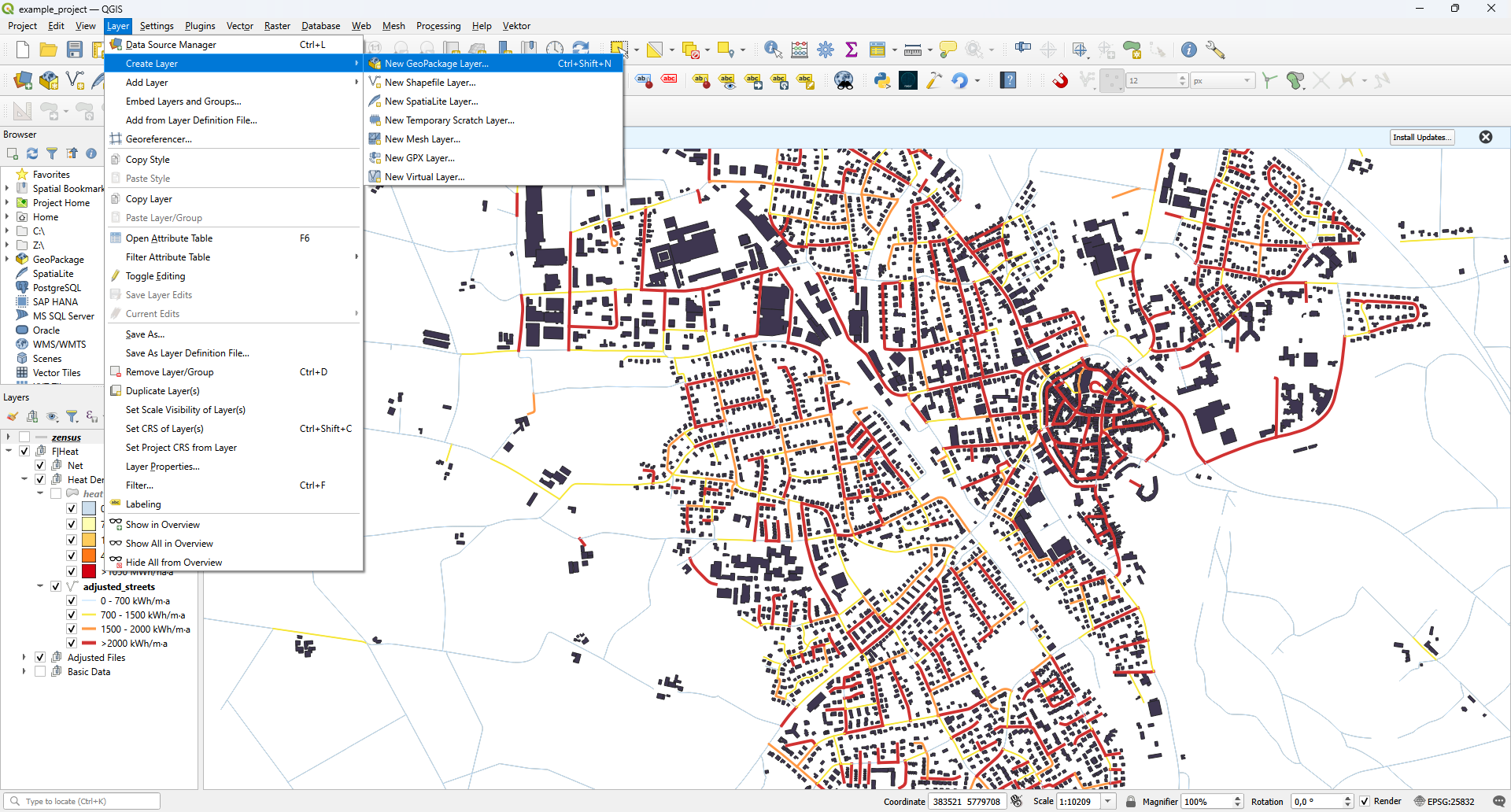
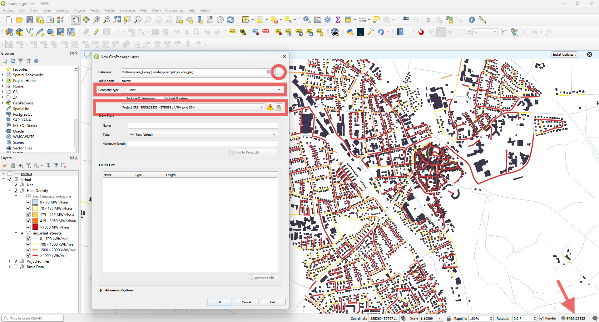
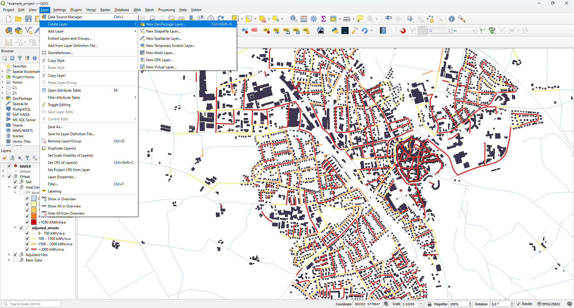
17. Before a heating network can be planned, you need to create a heat source and optionally define a planning area. You can create a new layer by selecting Layer > Create Layer > New GeoPackage Layer….

    

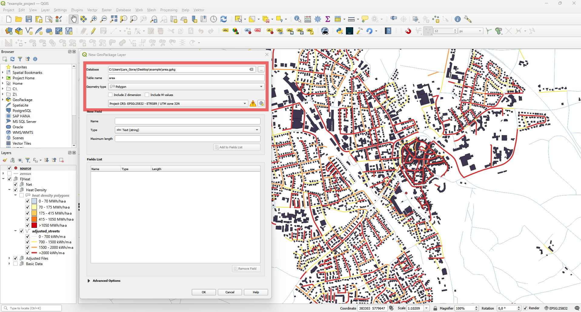
18. First we create the source. First set a file path by pressing the (…) button. Choose “Point” as geometry type. Make sure that you select the same coordinate reference system as your project. You can see your project’s CRS in the bottom right corner.

    

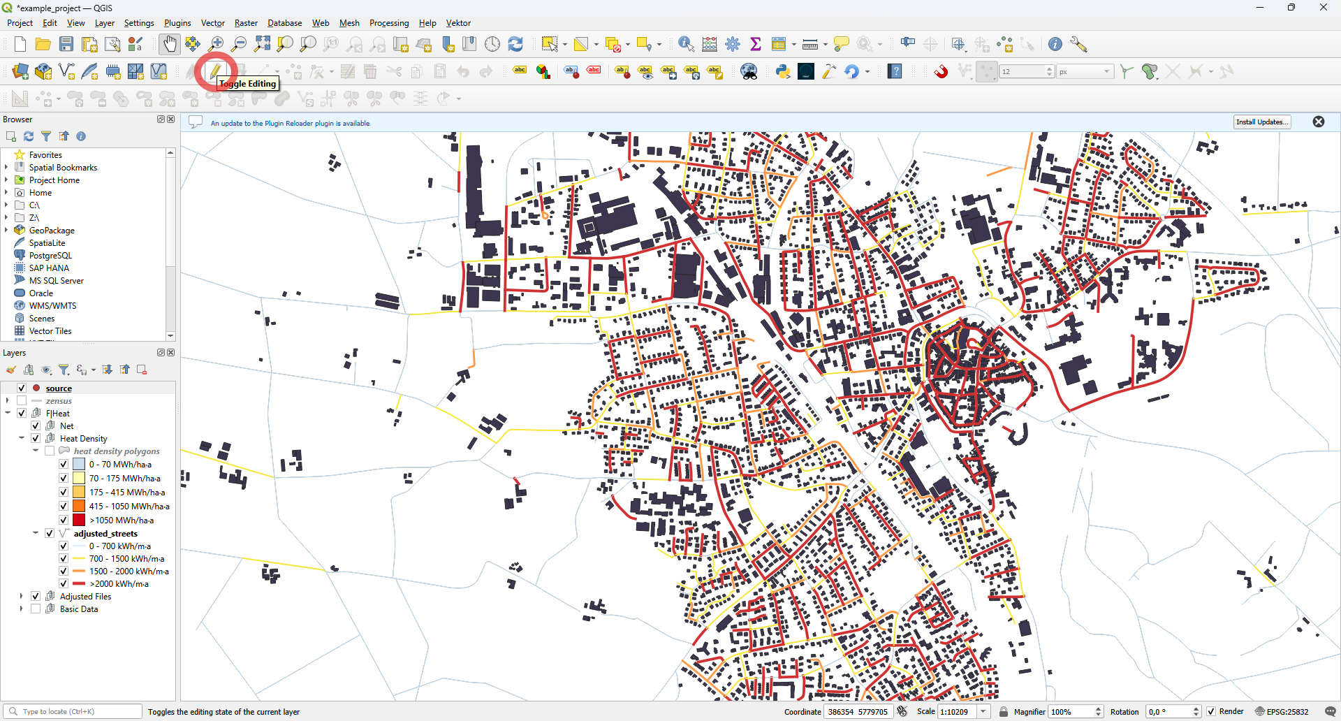
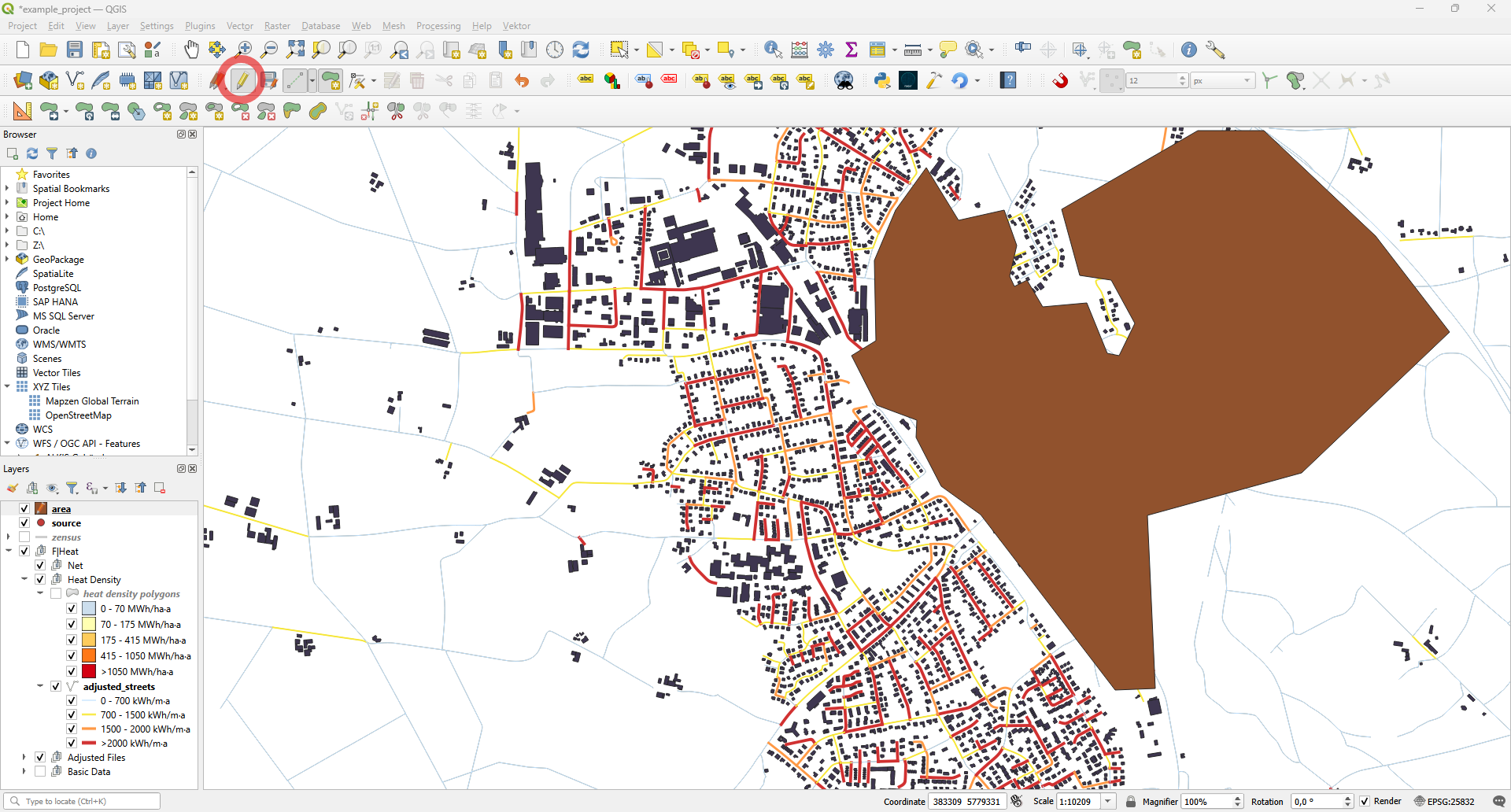
19. After you press OK, the new layer is added to your layer tree. Then you can press the Toggle Editing button.

    

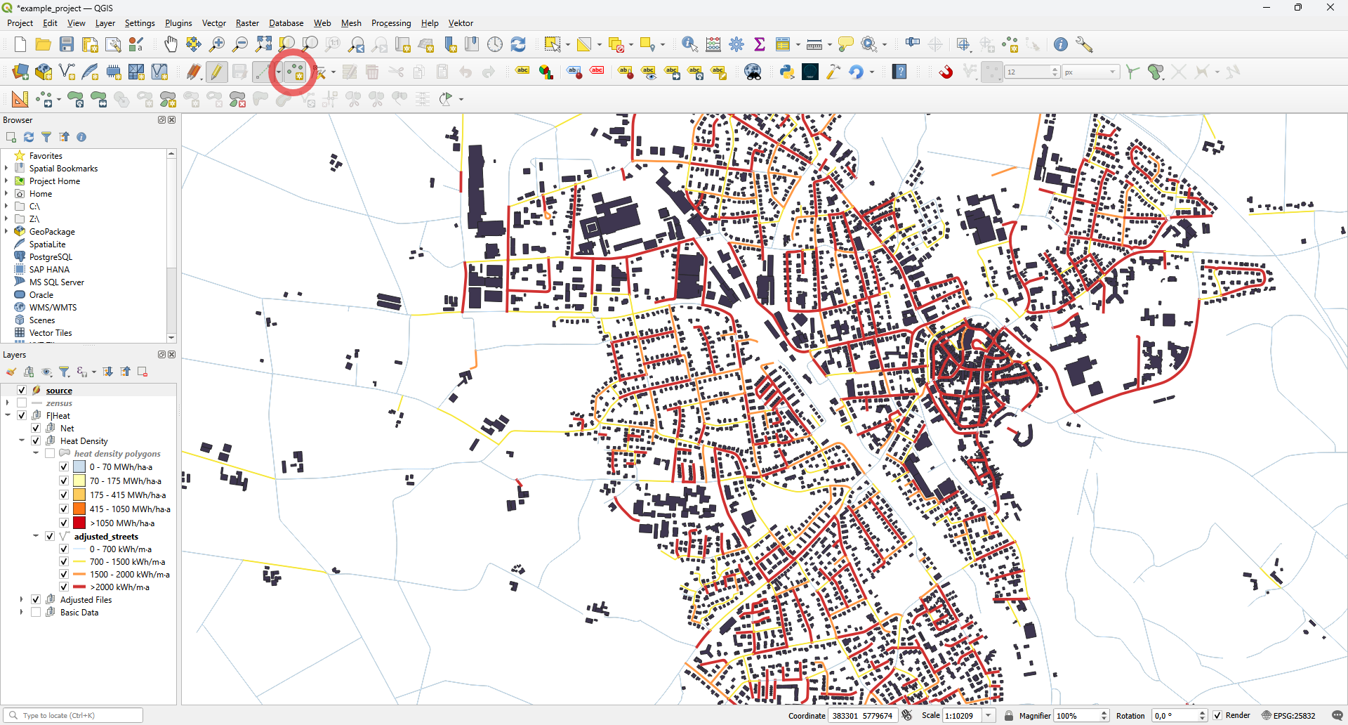
20. Press the Add Point Feature button and click on the map to place a point.

    

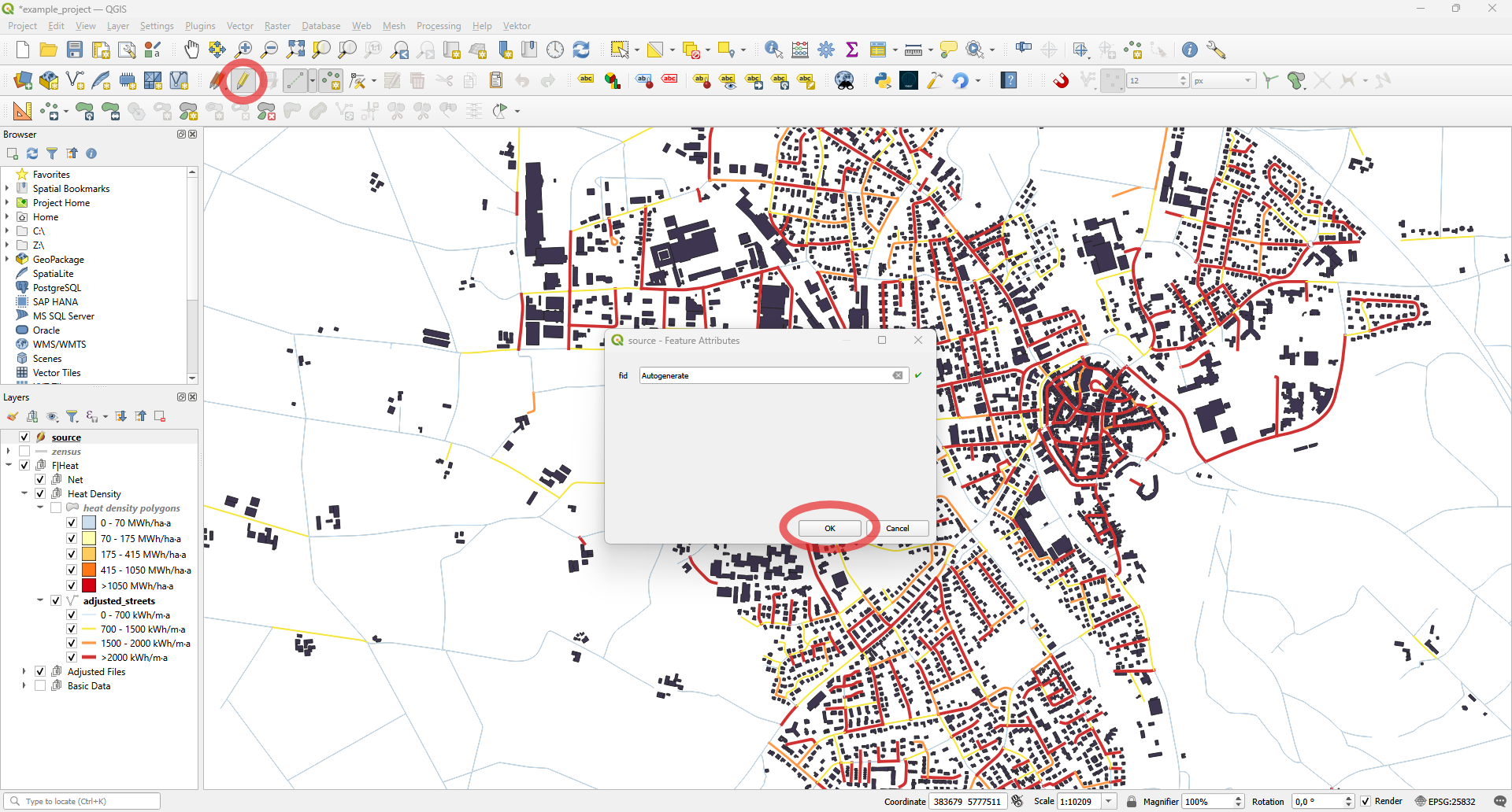
21. Simply press OK when the Feature Attributes window appears. Then exit edit mode and save the layer by pressing the Toggle Editing button again.

    

22. Create a new layer for the planning area.

    

23. This time, select “Polygon” as the geometry type. Again, set the correct CRS.

    

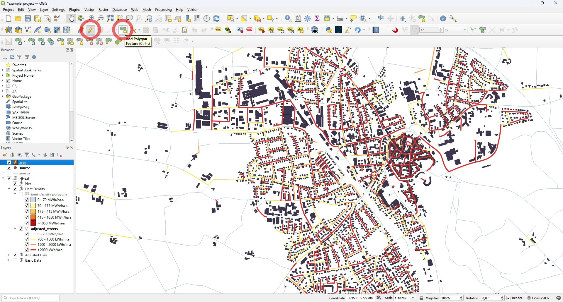
24. Press the Toggle Editing button and then select Add Polygon Feature.

    

25. The buildings you want in your planning area must be completely inside the polygon. Right-click to finish your polygon and press OK when the Feature Attributes window appears.

    

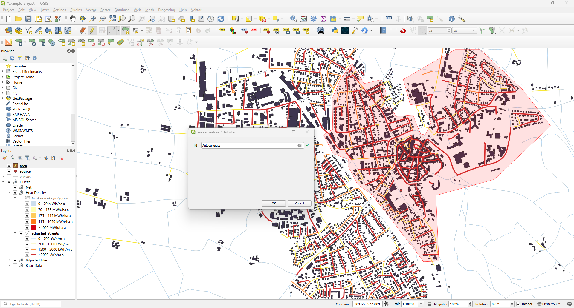
26. Exit edit mode and save the layer by pressing the Toggle Editing button again.

    

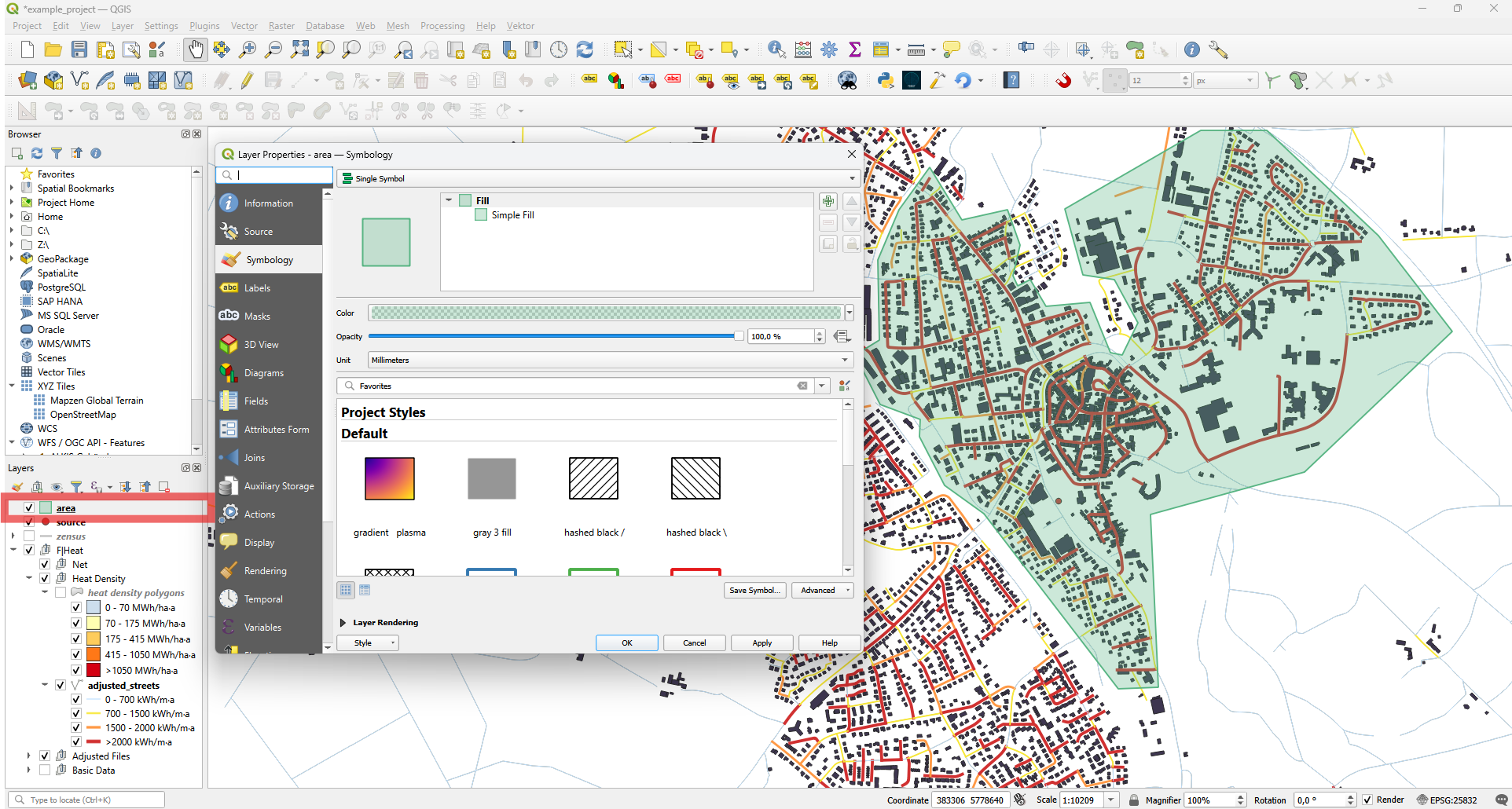
27. You can change the layer properties by double-clicking the layer. For example, you can adjust the color and opacity so that the buildings and streets remain visible. Alternatively, you can move the area layer down in the layer tree.

    

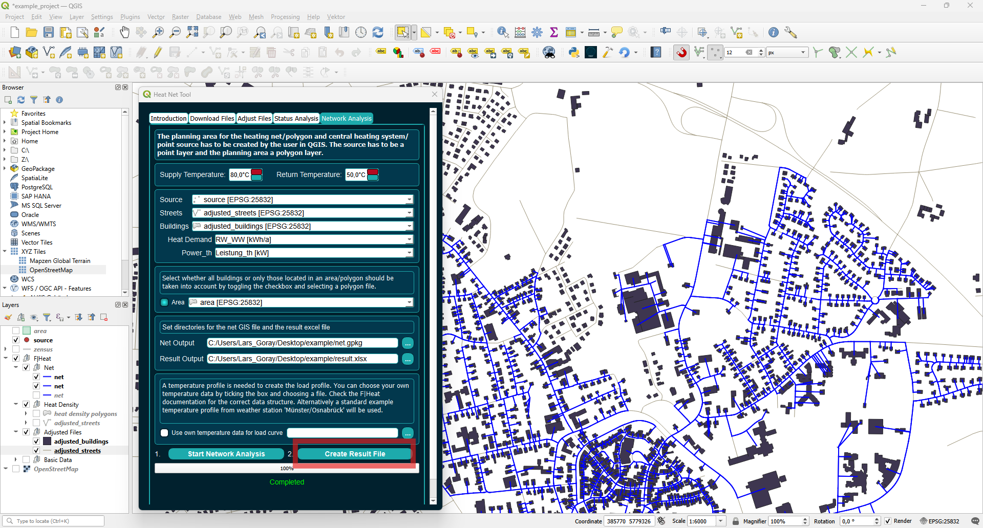
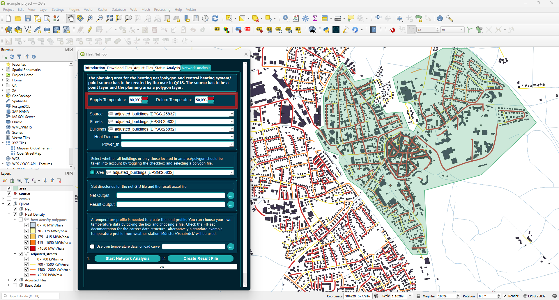
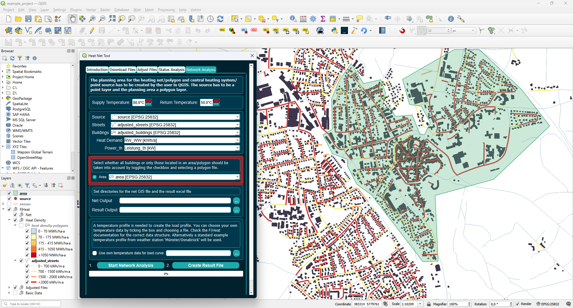
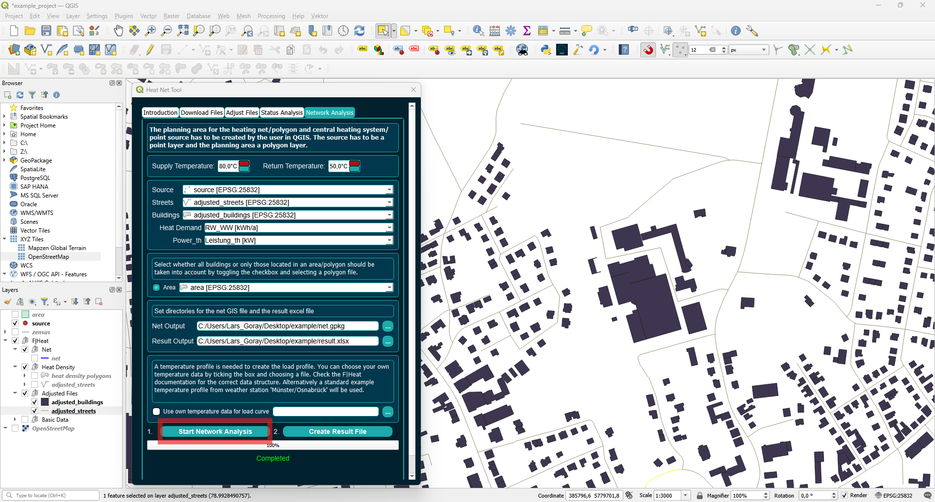
28. Now you can proceed with the planning in the Network Analysis tab. First, select the supply and return temperatures. The design is carried out for a district heating system within a specific temperature range. Anergy/LowEx networks and high-temperature/steam networks are not designed; therefore, for the flow temperature range, only values between 60 and 90 degrees Celsius can be selected. The return temperature must then be selected within the corresponding range.

    

29. Select your layers and attributes as in the previous steps.

    

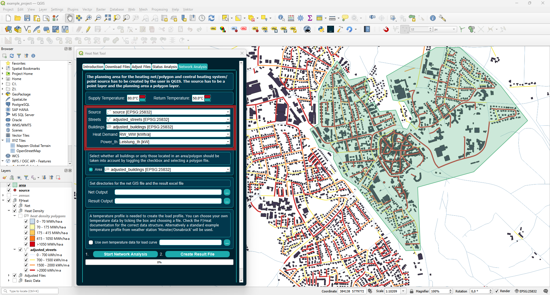
30. Select your planning area. Optionally, you can also choose to connect all the buildings from the building layer to your network by toggling the button on the left.

    

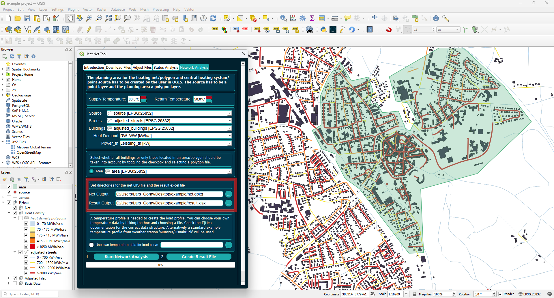
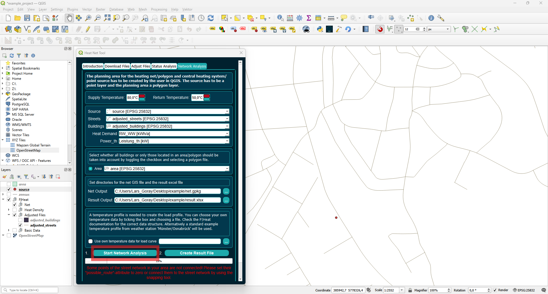
31. Set the file paths for the net GIS file and the result Excel file.

    

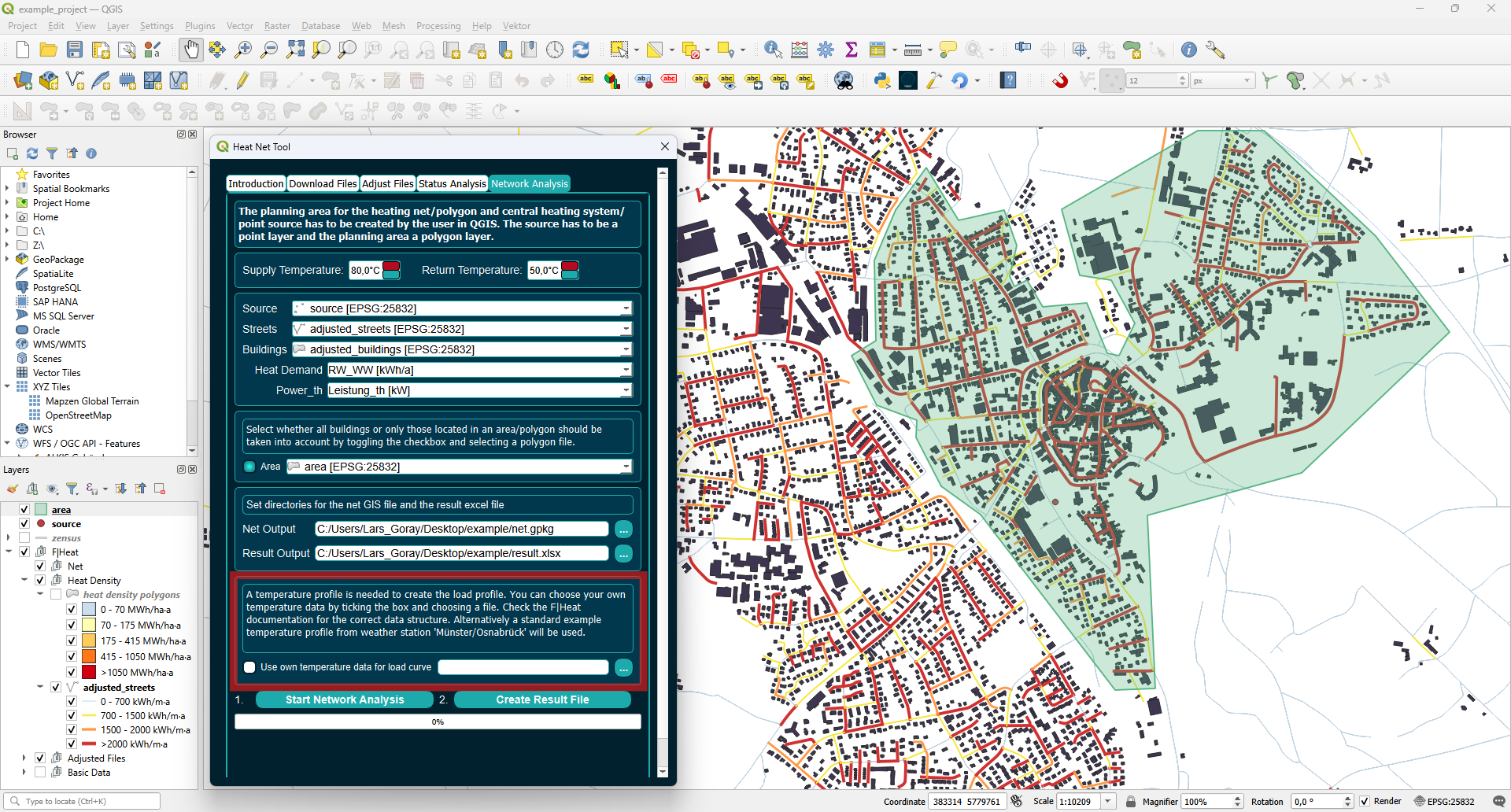
32. A temperature profile is needed to create the load profile. You can select your own temperature data by ticking the box and choosing a file. Alternatively, a standard example temperature profile from the weather station ‘Münster/Osnabrück’ will be used.

    

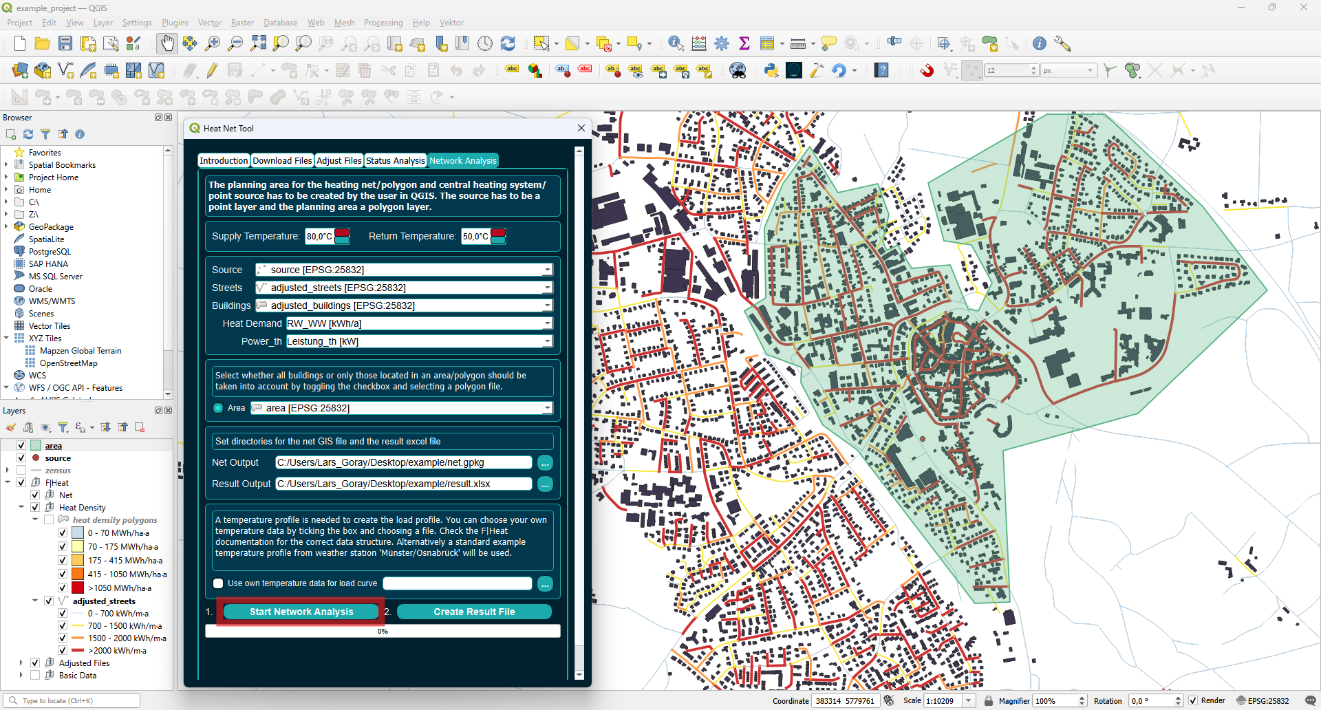
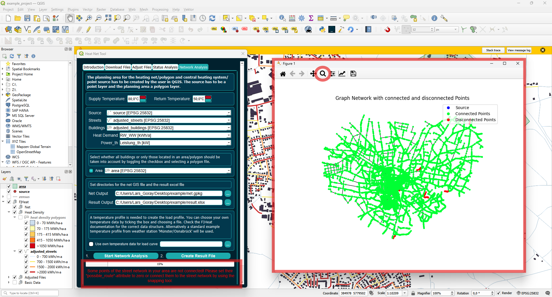
33. Press Start Network Analysis to start the process.

    

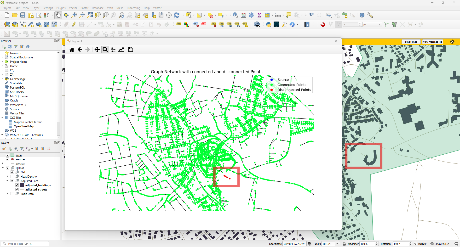
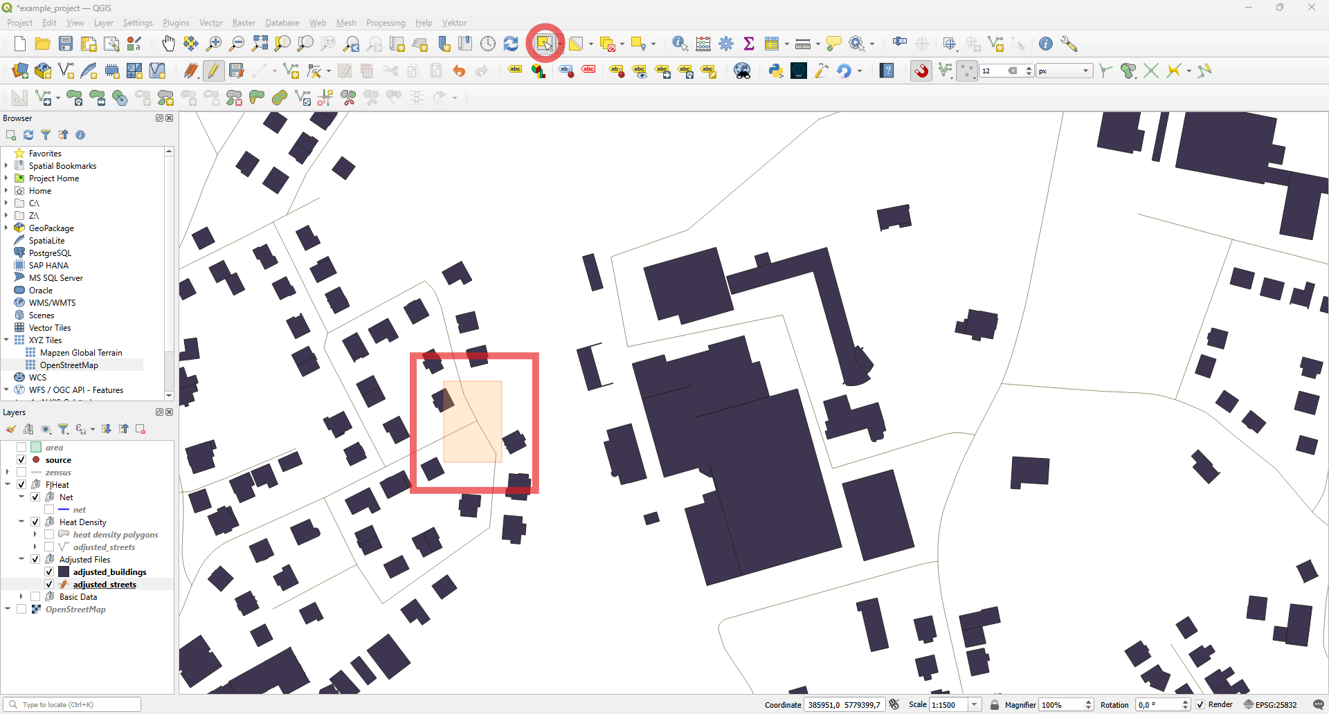
34. You may encounter an error indicating that some points of the street network in your area are not connected to the source. A figure showing the network of streets, buildings, and the source will appear. You can zoom in by pressing the magnifying button and drawing a rectangle.

    

35. Here we can see the disconnected street.

    

36. There are two options to fix this problem:

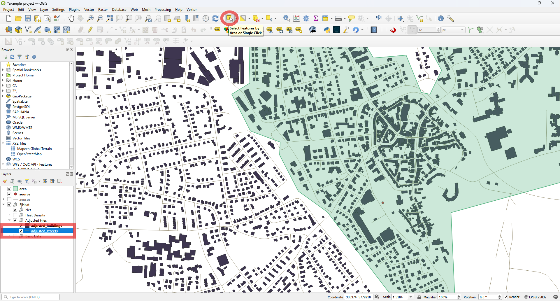
    1. Change the street’s attribute to be a possible route. The street will then be neglected, and the building will be connected to the next closest street.

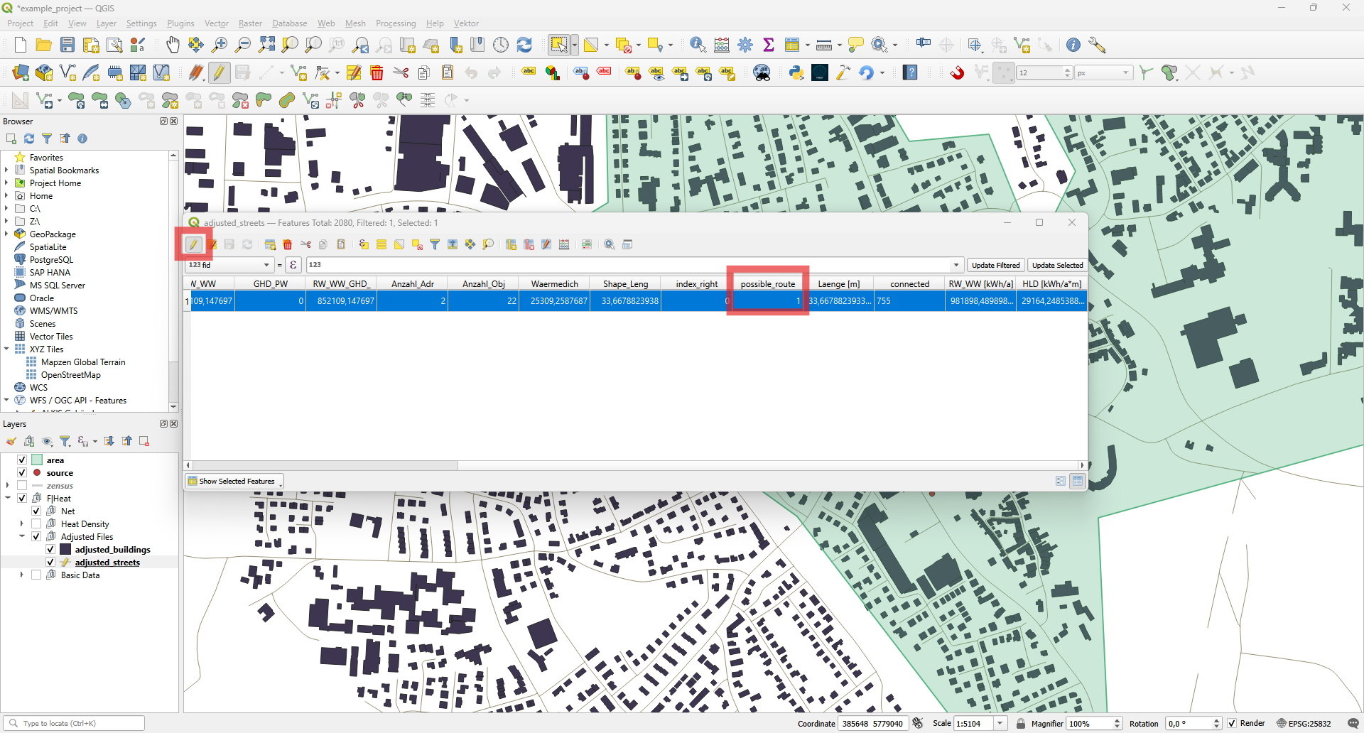
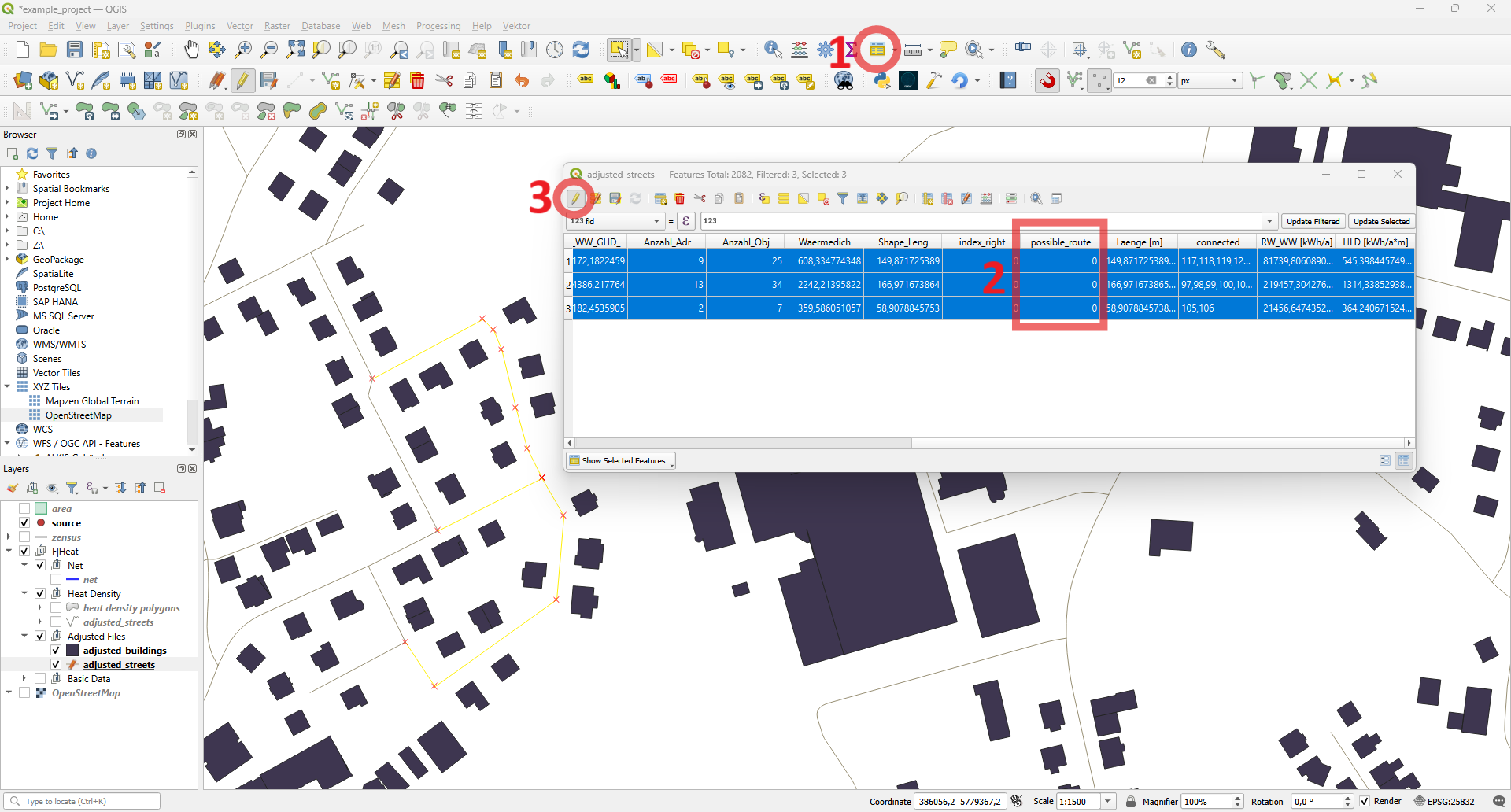
       Select the street layer and press the Select Features button to choose the disconnected street.

       

       Select the street and open the attribute table by right-clicking the layer or by pressing the Open Attribute Table (Selected Features) button.

       

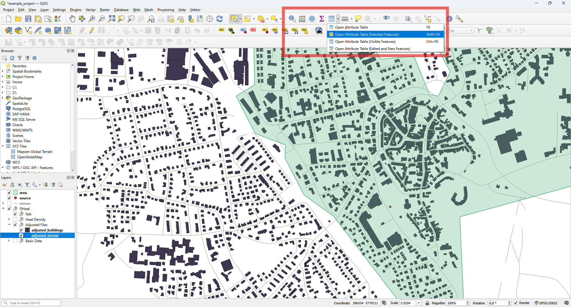
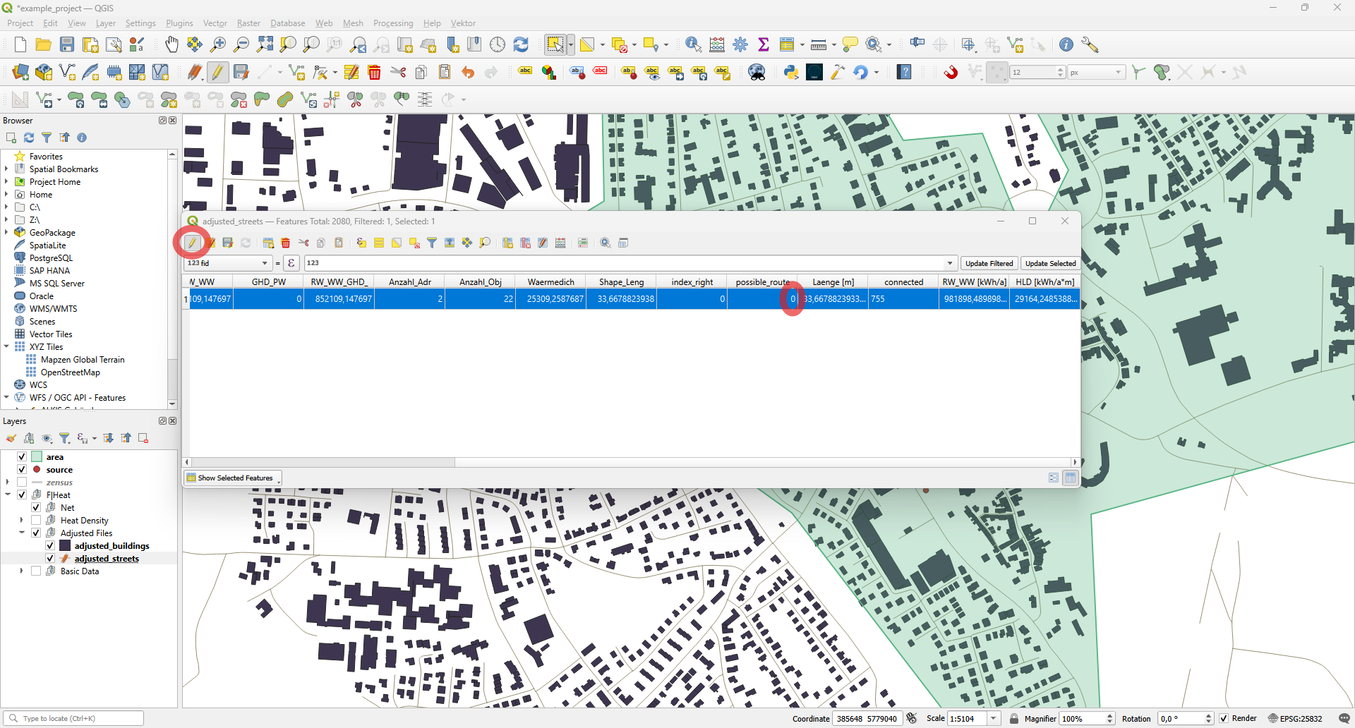
       Toggle editing mode and change the value under possible_route / Moegliche_Route from 1 to 0.

       

       Toggle editing mode again to save the changes to the layer.

       

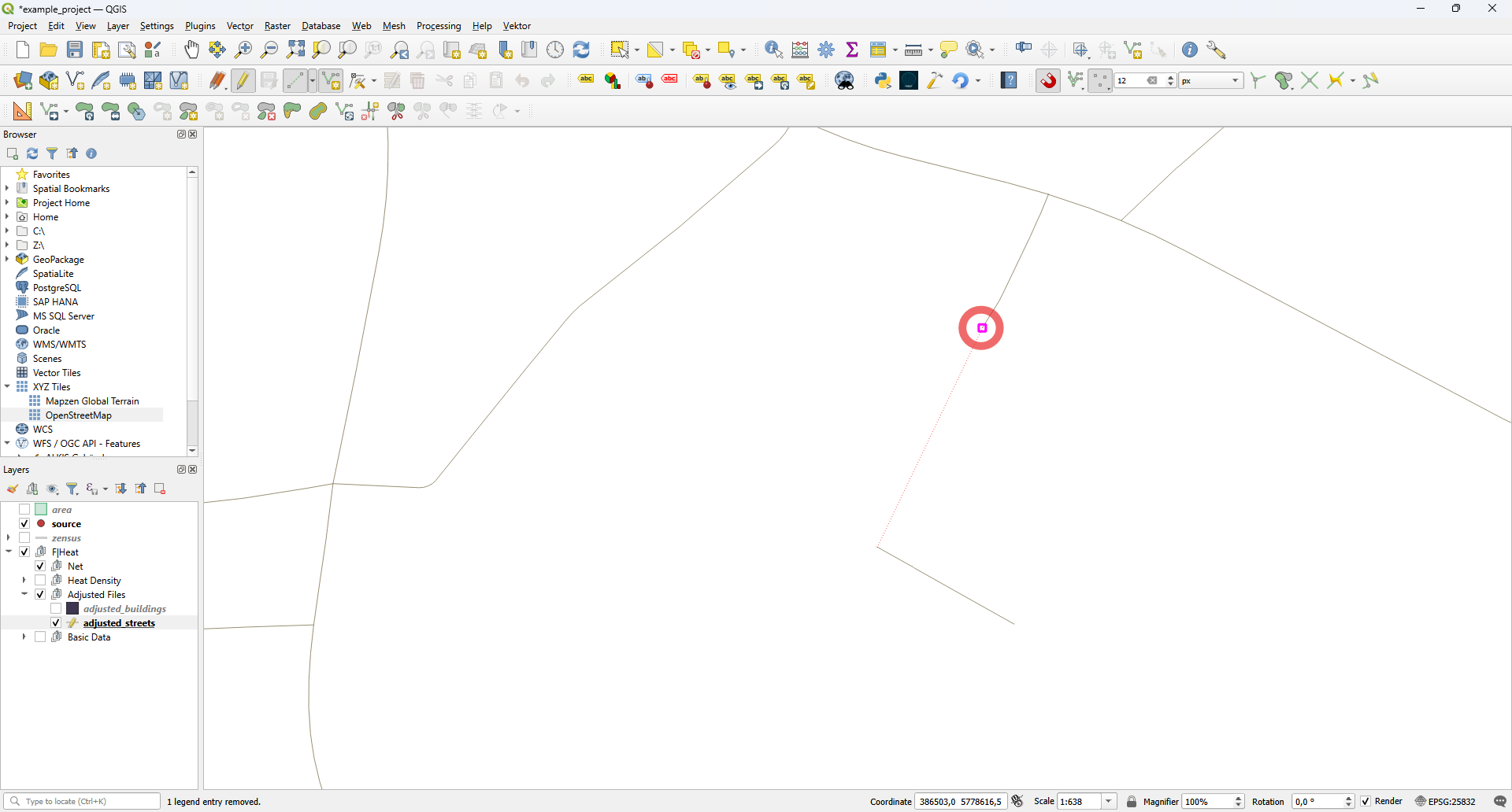
    2. Connect the street to the street network.

       Select the streets layer and toggle editing mode.

       

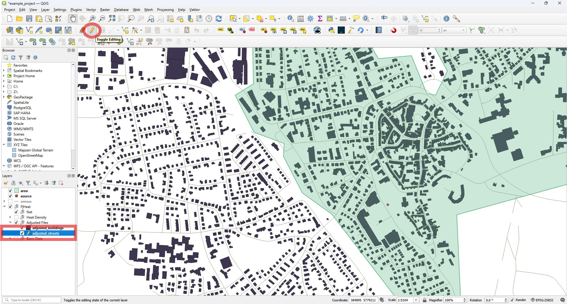
       Make sure snapping is enabled! Otherwise, the street will not be connected properly. Then press Add Line Feature to draw a new line connecting the street to the rest of the street network.

       

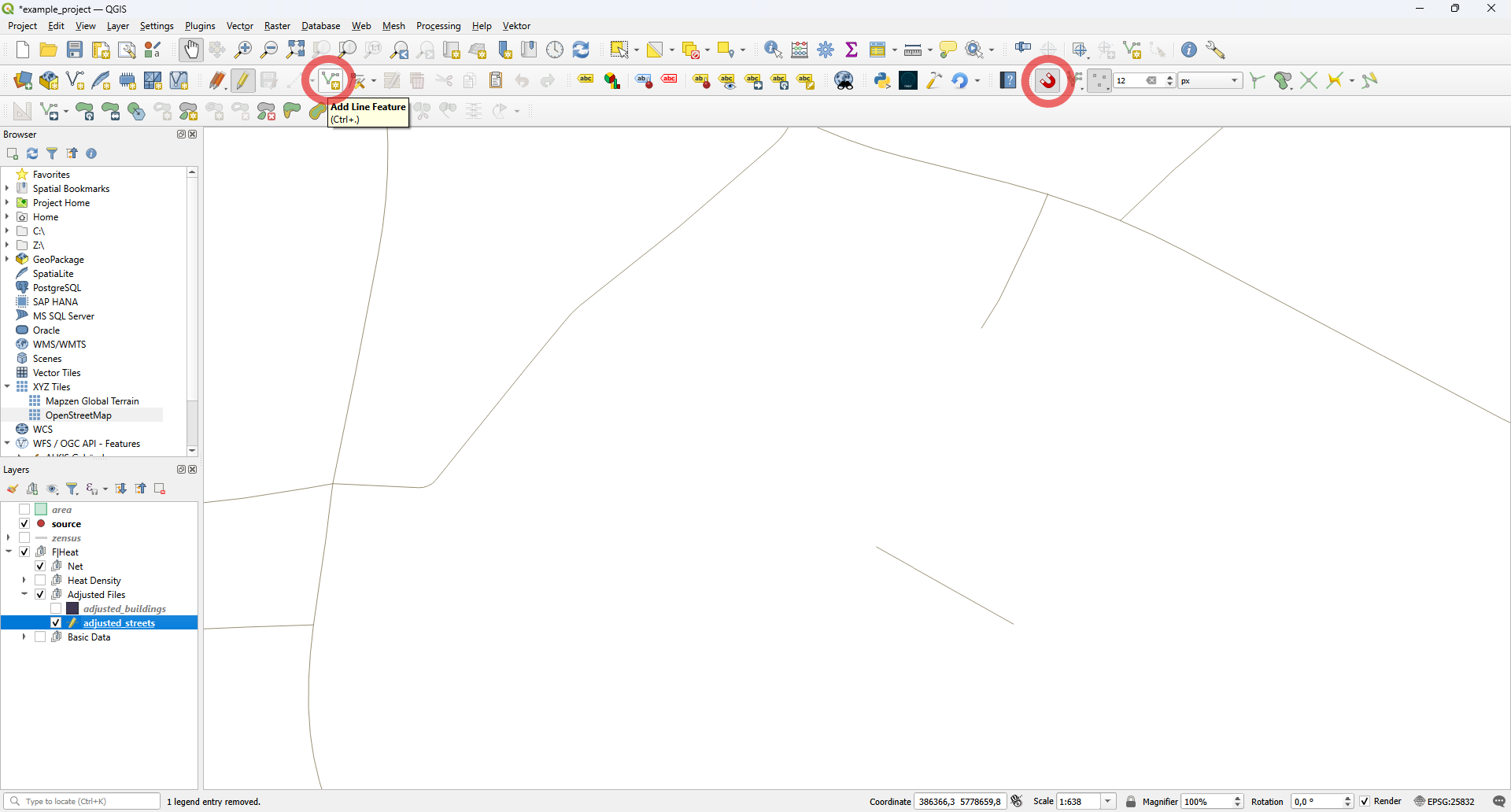
       Connect the streets. Thanks to snapping, the street points will be highlighted when you move the cursor close to them.

       

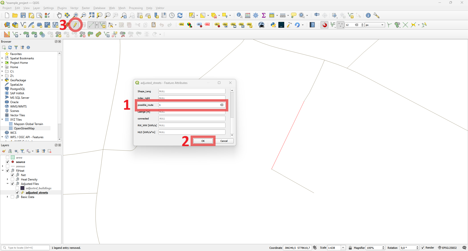
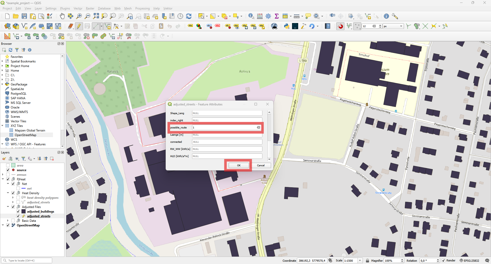
       Right-click to exit drawing mode. The Feature Attributes Window will appear. Scroll down and enter a 1 for the possible_route / Moegliche_Route attribute. Press OK and toggle the editing mode again to save the layer.

       

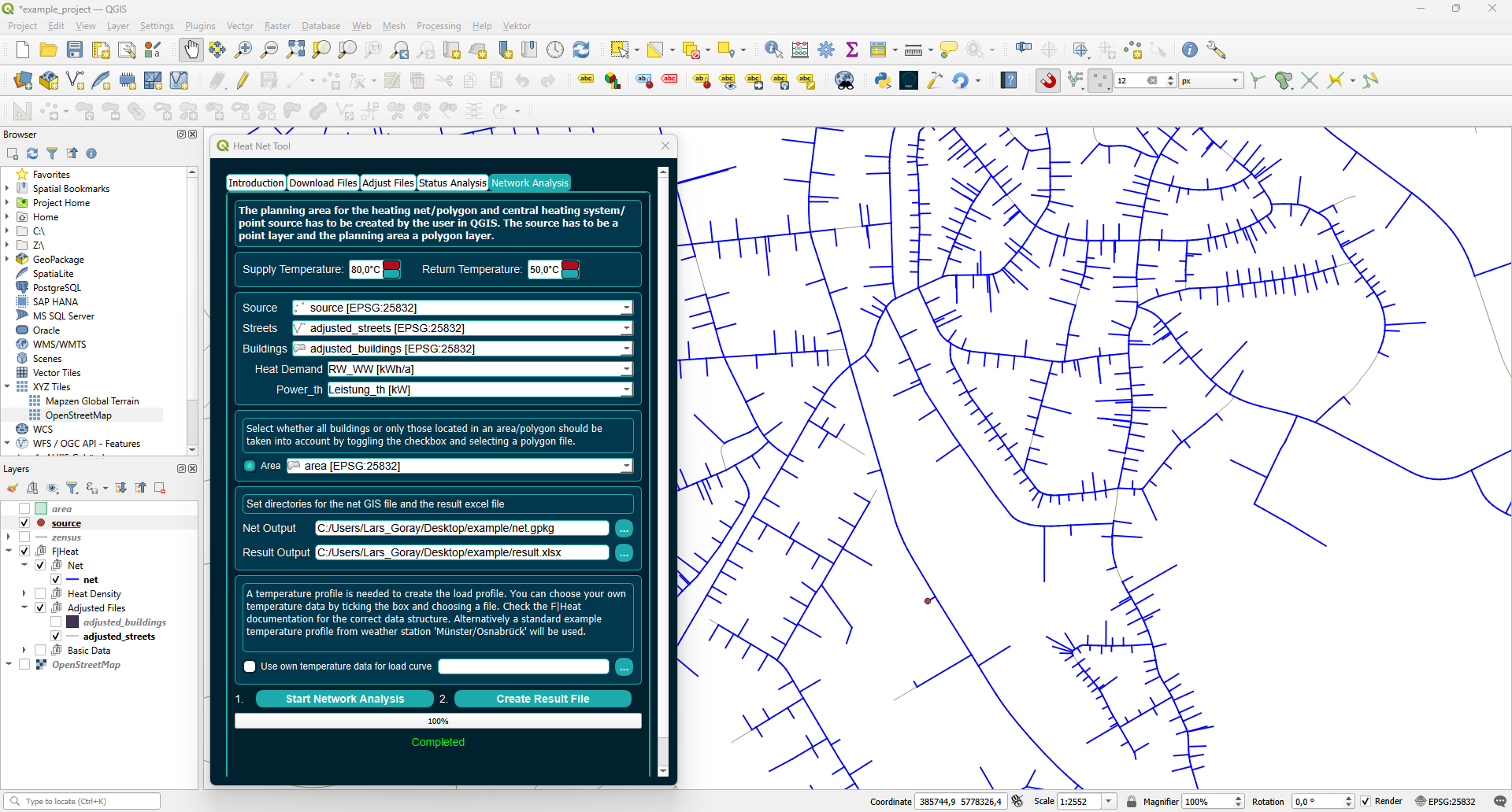
37. In this example, we have connected the street. Now we can start the network analysis again.

    

38. When the process is complete, the network is added to the layer tree.

    

39. You can check the network for paths that make little sense. Currently, the program only searches for the shortest path from the building centroid to the source, so some paths may not be optimal. Additionally, smaller streets may not be included in the street file and can be added manually. In this example, a path runs outside the network area. There are no buildings connected there, which makes this route very unfavorable.

    

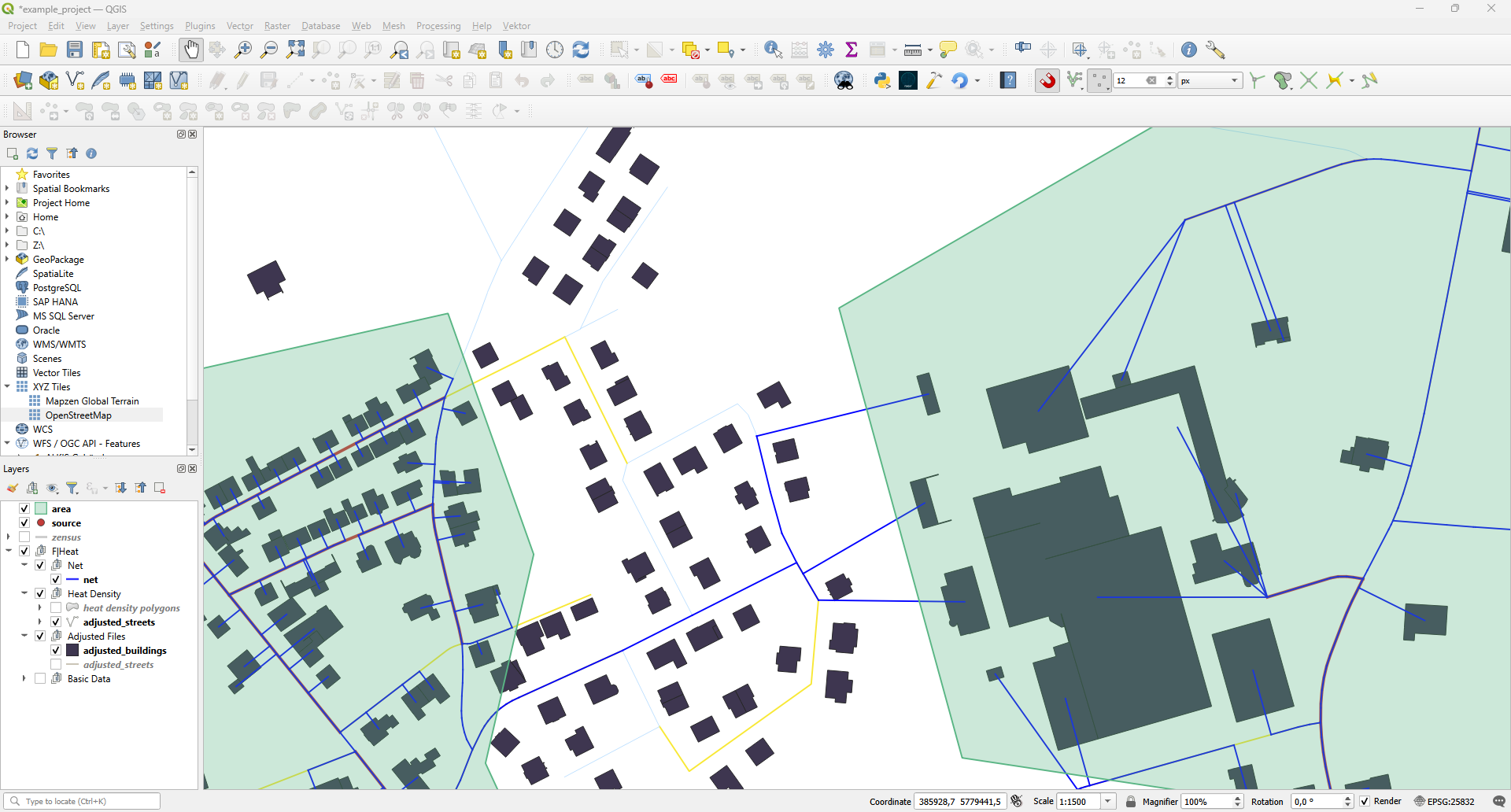
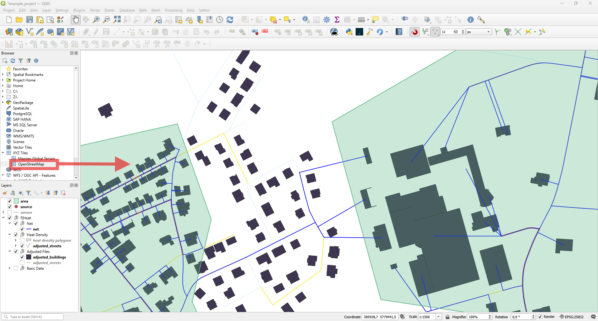
40. OpenStreetMap can assist you in adding new streets to the street layer. It can be found in the browser under XYZ Tiles. Simply drag and drop it into your project.

    

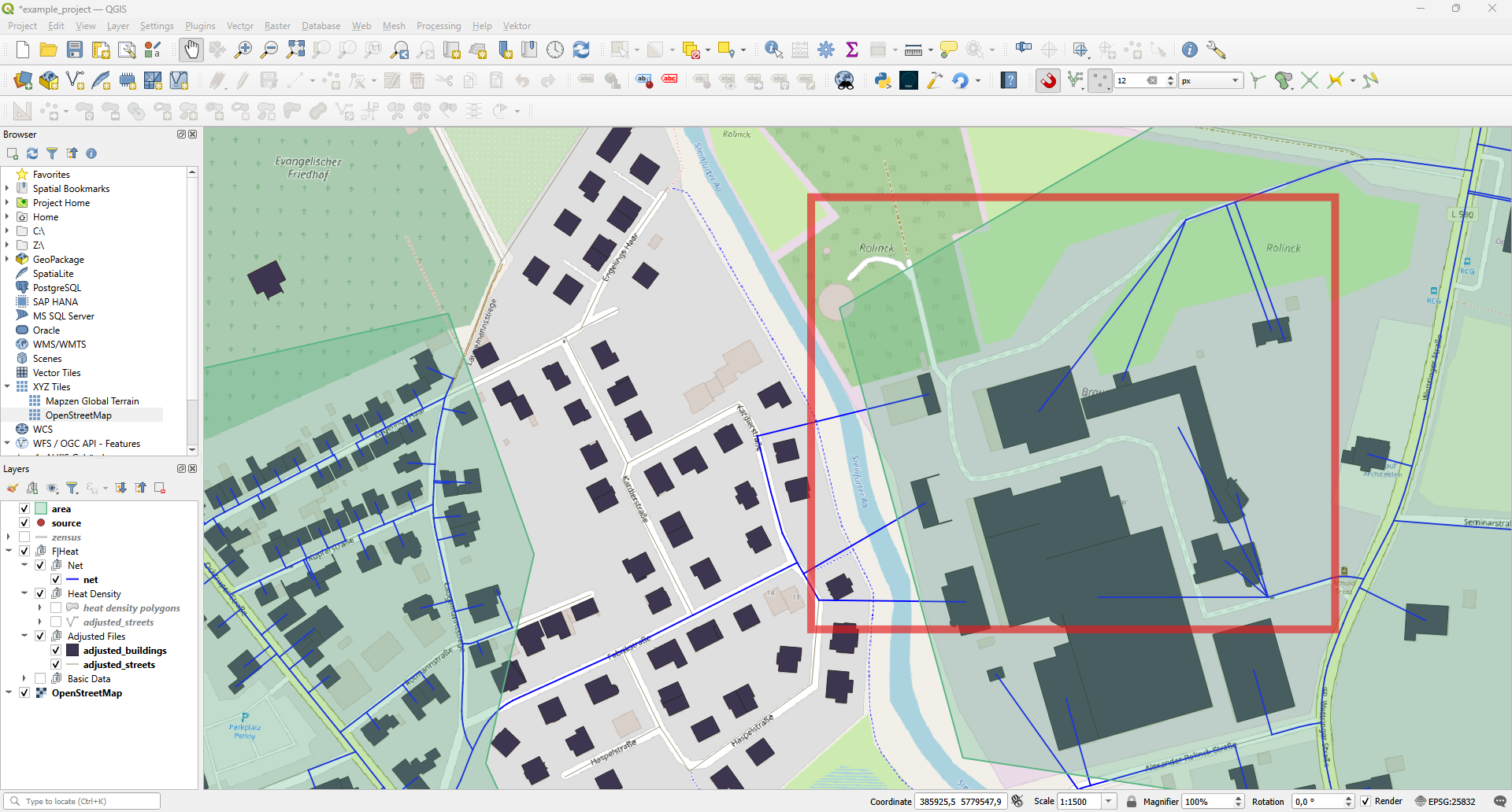
41. Now you can see that there are streets not included in the street layer.

    

42. You can easily add new streets like earlier when connecting the street to the street network:

    • Select the streets layer

    • Toggle Editing mode

    • Make sure that snapping is active

    • Add a new line feature (street)

    

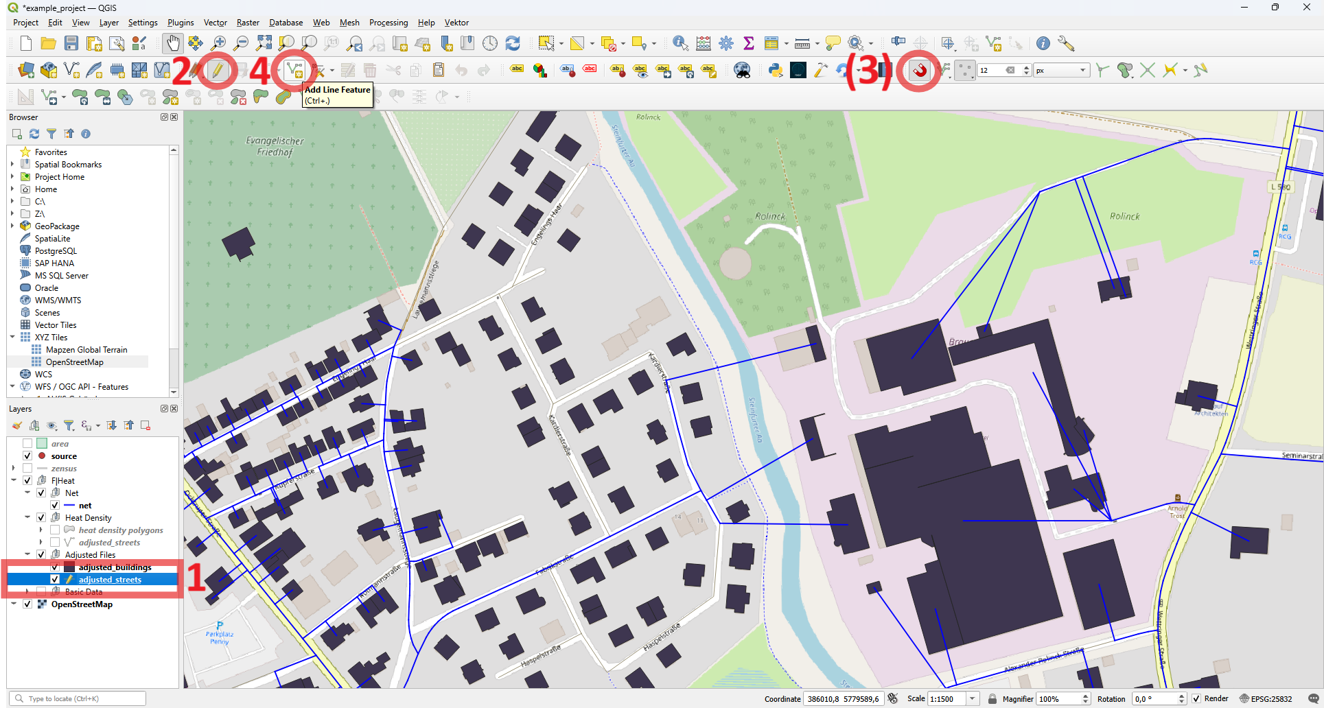
43. Follow the street and use snapping to connect it to a point in the street network.

    

44. Do not forget to enter 1 at possible_route / Moegliche_Route in the feature attributes.

    

45. In addition, we can select the nearby streets that we do not want to include as routes and enter 0 for their possible_route / Moegliche_Route attribute. Do not forget to toggle the editing mode once you are finished to save the layer.

    

    

    There are many more operations you can perform in QGIS, such as splitting line features, but it would be too much to cover all of them in this example. For more information, please refer to the QGIS Training Manual for more information.

46. Then you can start the network analysis again.

    

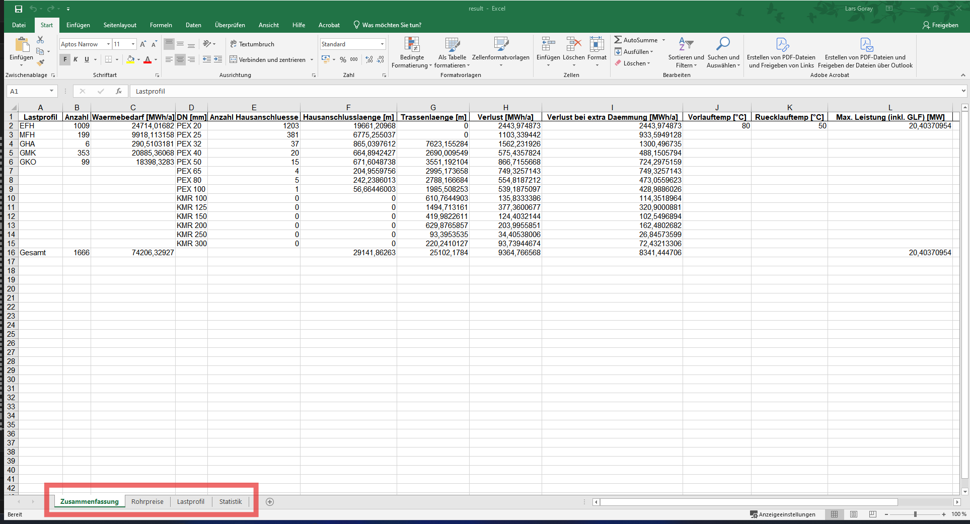
47. When you are satisfied with your heat network, you can create the result file. Once completed, the Excel file will open automatically, where you can find a net summary, pipe costs, load profile, and building statistics.